Lab 12: Path Planning and Execution

Objective and Considerations

The objective of this lab is to make the robot navigate through a series of waypoints, given as the following coordinates measured in feet:

1. (-4, -3)    <--start
2. (-2, -1)
3. (1, -1)
4. (2, -3)
5. (5, -3)
6. (5, -2)
7. (5, 3)
8. (0, 3)
9. (0, 0)      <--end

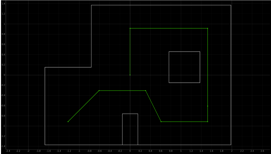
The map and path we need to navigate through is:

We are asked to complete this task using the method that is tailored best for the system that we have on hand. So, the first step is figuring out what is the best way to complete the task. To do this, I outlined several options to choose from, and evaluated their benefits versus their drawbacks. I also noted that each option didn’t have to be mutually exclusive – I could mix and match for certain waypoints if I thought a method would work better at specific locations.

Option 1: Open Loop Timing

The first and simplest option is to navigate to the waypoints completely using open loop. To do this, I would implement methods to navigate between every waypoint to the next, manually adjusting the turn and distance timings.

Pros:

• Simplest and requires no additional implementation.
• Can be tested faster and more easily since I don’t have to get the entire run all at once to implement each step. This could free up room in the lab as more people need the world to test their robots.

Cons:

• Extremely sensitive to changes in battery level and floor roughness.
• Timing each step manually may take longer than just implementing something more complex to handle several steps at once.

Option 2: Naive Waypoint Following

Next, I considered using onboard compute resources to calculate the required heading and turn angle to get from one waypoint to the next. This would be a relatively simple geometric calculation – I would fix the starting angle, then assume that the robot turns by precisely the angle needed and travels exactly the distance needed. For example, from waypoint 0 to waypoint 1, I would hope for it to turn 45 degrees, then travel exactly 2*sqrt(2) ft.

Pros:

• Does not require manually tuning the timing for each step.
• Low compute cost onboard.
• Still very fast.

Cons:

• Somewhat sensitive to variations in environment and battery level (less than open loop since changes invalidate one overarching algorithm rather than 8 distinct timings).
• Will not complete if, at any step, the robot does not travel exactly the angle and distance calculated.

Option 3: Using TOF Readings Directly

Then, I considered ways to use TOF data to guide stopping distances. To do this, I could either use straight-line trajectories or travel exclusively with 90-degree turns.

For straight-line motion, I would have to cast a ray from each waypoint to the next and find out what distance the TOF expects to see. For certain pairs (e.g. waypoint 0 to waypoint 1), that distance ends up being rather large.

Pros (straight-line):

• Incorporates sensor readings and is more robust to small deviations in robot behavior (more so in the forward-backward dimension and not so much if there is rotational variance).

Cons (straight-line):

• For faraway distances, slight changes in angle can drastically impact reading (e.g. waypoint 0 to waypoint 1 – a slight clockwise rotation would cause TOF to read the square obstacle rather than the top wall).
• Relies greatly on TOF sensor accuracy and precision, which at faraway points can be hazy. Poor precision will cause the linear PID to become unstable even if it is reading the expected value. Poor accuracy will cause stopping at an incorrect location.
• Requires PID tuning – and perhaps different tunings may work better for different stopping distances.

For grid-like motion, I would instead break up diagonal movements on the map into two 90-degree movements. This ensures that the TOF would read against a wall that is perpendicular to the light ray casted.

Pros (grid):

• Incorporates sensor readings and TOF will be less sensitive to angle deviations.

Cons (grid):

• Execution will be much slower since path is not optimal.
• This method becomes impossible if the map requires diagonal movements, or impractical if the map is too congested and non-optimal paths increase risk of collision by a significant amount.

Option 4: Localization

Finally, the most heavy-duty approach would be to execute localization and compute a belief of where the robot is in the world. The computation of belief would use a Bayes filter on a laptop, communicating with the robot live using BLE. Instead of assuming its position, the robot could have a better probablistic grasp of where it is and correct its own position as necessary.

Pros:

• More robust algorithm: can adjust to imperfections in motion.

Cons:

• Takes a massive amount of time to execute. This may not matter so much if I was doing this lab as a hobbyist but it certainly is a factor to consider when you (and 60 frustrated classmates) have to finish the lab with a busy finals schedule!
• Communication can disconnect mid-run, which may require a backup plan to be implemented. If the robot is midway through correcting its position via localization output, it will likely be unable to resume.

Chosen Method

Once I considered all of the options, I chose to combine my options based on what I expected to work on my robot.

First, I discarded the idea of using localization because I thought it was too heavy-duty of a tool for the job. Since we are given the waypoints ahead of time, we never need to use our current position to plan out a path, except for correcting its position back to a waypoint. And given that we have open access to the world and can reset our robot rather quickly, the time that it would take to execute the localization far exceeds if I just picked up my car and tuned its parameters with a simpler method. If the localization algorithm was faster on my robot, or if there were dynamic obstacles that I needed to avoid during the run, I would have definitely implemented it. But as it stands, I did not think localization was worth using for this task.

Then, I eliminated using complete open loop because of how unreliable it is. I could have the timings perfect to go from the middle of one waypoint to another, but even then all of it could fall apart when I traverse all 8 waypoints in sequence. Tuning all 8 paths by hand would also take way too much time, especially if repeated testing drains the battery levels and causes the car to go slower.

With that being said, I ended up combining naive waypoint traversal and TOF readings. I wanted to calculate the turn angle and travel distance onboard, but reserve the ability to use the TOF sensor to ensure that the robot is able to stop at a specified distance. This becomes really useful for tighter regions like the bottom-right corner of the map. On top of that, I could then adjust the TOF thresholds to counteract when the robot builds up too much momentum during longer distances.

Implementation

For my implementation, I wanted to ensure modularity and generalizability just in case I wanted to change the details of the implementation (e.g. incorporate a probablistic update to robot’s position belief) further down the line.

Planner (Naive)

For the planner, I need to:

1. Be able to receive a series of waypoints
2. Calculate the heading and distance to head to the next waypoint.

To do this, I define a new module with a Planner class:

planner.hpp:

#ifndef PLANNER_HPP
#define PLANNER_HPP

#include <vector>
#include <cmath>

struct Pose
{
  double x;
  double y;
  double theta; // In degrees
};

struct Waypoint
{
  double x;
  double y;
};

class Planner
{
public:
  Planner(const std::vector<Waypoint> &waypoints);

  double calculateHeadingToWaypoint(const Pose &currentPose, int waypointIndex) const;
  double calculateDistanceToWaypoint(const Pose &currentPose, int waypointIndex) const;

private:
  std::vector<Waypoint> waypoints_;
};

// Extern declarations for global var.
extern Planner planner;
extern const std::vector<Waypoint> waypoints;
extern const int numWaypoints;
extern float stoppingDistances[];

#endif // PLANNER_HPP

planner.cpp:

#include "Planner.hpp"

const std::vector<Waypoint> waypoints = {
    {-4.0, -3.0}, // Start
    {-2.0, -1.0},
    {1.0, -1.0},
    {2.0, -3.0},
    {5.0, -3.0},
    {5.0, -2.0},
    {5.0, 3.0},
    {0.0, 3.0},
    {0.0, 0.0} // End
};
const int numWaypoints = 9;

// Corresponds to the waypoints' order
float stoppingDistances[] = {
    0.0, // waypoint 0
    0.0, // waypoint 1
    0.0, // waypoint 2
    0.0, // waypoint 3
    1.0, // waypoint 4 --> early stop: bottom right corner
    0.0, // waypoint 5
    2.0, // waypoint 6 --> early stop: top right corner
    3.0, // waypoint 7 --> early stop: above origin
    0.0  // waypoint 8
};

// Define the global Planner using the waypoints
Planner planner(waypoints);

Planner::Planner(const std::vector<Waypoint> &waypoints)
    : waypoints_(waypoints) {}

double Planner::calculateHeadingToWaypoint(const Pose &currentPose, int waypointIndex) const
{
  if (waypointIndex < 0 || waypointIndex >= waypoints_.size())
    return 0.0;

  const Waypoint &wp = waypoints_[waypointIndex];
  double dx = wp.x - currentPose.x;
  double dy = wp.y - currentPose.y;
  double targetAngle = std::atan2(dy, dx) * 180.0 / M_PI; // radians to degrees

  double deltaTheta = targetAngle - currentPose.theta;
  while (deltaTheta > 180.0)
    deltaTheta -= 360.0;
  while (deltaTheta < -180.0)
    deltaTheta += 360.0;

  return deltaTheta;
}

double Planner::calculateDistanceToWaypoint(const Pose &currentPose, int waypointIndex) const
{
  if (waypointIndex < 0 || waypointIndex >= waypoints_.size())
    return 0.0;

  const Waypoint &wp = waypoints_[waypointIndex];
  double dx = wp.x - currentPose.x;
  double dy = wp.y - currentPose.y;
  return std::sqrt(dx * dx + dy * dy);
}

The waypoints vector is defined as a const value in this code, but it can be changed to dynamically receive the waypoints from bluetooth if I needed, without disturbing the calculating methods attached to it. I could also instantiate the class with different sets of waypoints.

Executing the Plan

To execute the plan, I need to be able to:

1. Turn by an angle delta – the difference between required heading and current DMP heading.
2. Travel by distance d calculated by the planner.

To do this, I added these building block functions to my motor-driving module:

Turning:

void rotateByAngleWithPid(float angle)
{
  // timeout for PID at each step. We assume that each turn will not exceed this time.
  const int timeout = 2000;

  unsigned long startTime = millis();

  float heading = getValidDmpYaw(); // Delays until a valid DMP reading is ready
  angle_pid.setSetpoint(heading + angle);

  while (millis() - startTime < timeout)
  {
    heading = getValidDmpYaw(); // Delays until a valid DMP reading is ready
    int pwm = angle_pid.compute(heading);
    executeAnglePid(pwm);
  }
  stop();
  angle_pid.resetAccumulator();
}

My turning code turns strictly for 2 seconds at each waypoint, which I found to be a safe amount of time for oscillations to settle in my angular PID. I could have reduced it even more, but I used a more lenient time to debug an error that I had with my angular PID since speed was not a major objective in this lab (my derivative term was using a powerful low pass filter, causing it to not dampen my oscillations…).

Driving:

float motorSpeed = 5; // ft/sec, measured via straight line test

// Let sd = stoppingDistances[waypointIndex]; 
// If sd != 0, the TOF is checked to see if its reading < sd + some buffer distance, and stops if so.
// It does this by breaking up the forward travel into discretized timeStep (seconds) chunks.
void driveForwardDistance(float dist, int waypointIndex)
{
  const float timeStep = 0.01; //s
  const int stepDelay = int(timeStep * 1000); //ms
  float totalTime = dist / motorSpeed;

  drive(FORWARD, 150);
  unsigned long start = millis();

  float stopDistanceFeet = stoppingDistances[waypointIndex];
  bool shouldCheckTof = (stopDistanceFeet > 0.0);

  while ((millis() - start) < (int)(totalTime * 1000))
  {
    delay(stepDelay);

    if (shouldCheckTof)
    {
      // Include motor stopping distance, esp if momentum (through testing: +1.5 feet extra)
      float bufferFeet = (stopDistanceFeet >= 2.0) ? 1.5 : 0.25;
      float stopThresholdMM = (stopDistanceFeet + bufferFeet) * 304.8;

      if (isTofUnder(stopThresholdMM))
      {
        Serial.print(stopDistanceFeet);
        Serial.println(" ft: TOF stop triggered early.");
        break;
      }
    }

    BLE.poll(); //to prevent disconnect
  }

  brakeFor(1000);
  stop();
}

This driving function drives a set distance while keeping the motor speed and stopping distances adjustable.

Putting it all together:

void executeWaypointSequence()
{
  Pose currentPose;

  // Start position: (x, y, theta=0) facing right
  currentPose.x = waypoints[0].x;
  currentPose.y = waypoints[0].y;

  for (int i = 1; i < numWaypoints; ++i)
  {
    BLE.poll(); // prevents disconnect
    currentPose.theta = getValidDmpYaw(); // degrees

    float angleToRotate = planner.calculateHeadingToWaypoint(currentPose, i);
    rotateByAngleWithPid(angleToRotate);

    float distanceToTravel = planner.calculateDistanceToWaypoint(currentPose, i);

    // Only check TOF early-stop at waypoint index 4 and 6
    driveForwardDistance(distanceToTravel, i);

    currentPose.x = waypoints[i].x;
    currentPose.y = waypoints[i].y;
  }
}

This code runs through the waypoints and executes them in order. Note that ++i pre-increments in the index so that in the body of the loop, i always points to the index we are navigating to. The last two lines update the current pose to be the waypoint the robot just arrives at, which could have been swapped out with a call to a localization function instead.

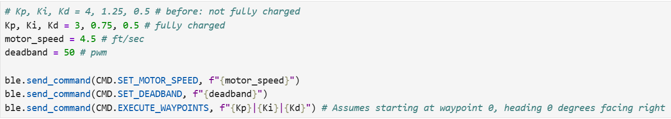
Starting the routine was done over bluetooth, using a command that sets the angular PID gains and calls this function.

Tuning Parameters: How Not To Pull Your Hair Out

Since my chosen method requires adjusting timings and tuning angular PID, a huge part of successfully executing the lab was implementing methods to quickly change my parameters.

For motor speed, I implemented a method to test motor speed, which is simply driving forward for 1 second before braking:

void driveForwardFor1Second()
{
  drive(FORWARD, 150);
  delay(1000);
  brakeFor(500);
  stop();
}

Using the tiles in the lab as 1-foot measurements, I could place the car down and call this function via bluetooth to get a good estimate of the speed.

Another issue I had during Lab 6 was having to reupload the code to change the value of my deadband. I also added a bluetooth function to change that value after changing DEADBAND from a #define macro to a global int value instead.

Finally, as mentioned earlier, I bundled specifying P, I, and D gains in the bluetooth call to start the waypoint execution sequence. It may seem small, but the combination of these quality of life bluetooth commands made the lab much more tolerable.

Results and Adjustments

Leading up to the best run I had, I will show several key runs and the adjustments I made at each point.

First few runs: unstable angular PID

The angular PID was constantly becoming unstable for even small rotations. This problem plagued a lot of my earlier runs. To fix this, I ended up having to run the waypoint sequence with the PID outputs printing to serial. It was only then I realized my derivative terms drastically lagged behind the rest of the controller, leading me to disable the low pass filter that I had inadvertently put on my derivative term.

Next set of runs: overtraveling distance and crashing:

For the next series of runs, my car was crashing into the end of the long distance from the bottom right to top right corners. I suspected it was because the car was traveling too fast. Checking the TOF for the intended stopping distance meant it was already too late to brake. To fix this, I had to add the buffer distance addition in my driving function.

Final tuning: slight overshoot:

For the last few runs, I was seeing my car not crash into the wall due to the buffer distances, but still overshooting. It was particularly strange because even though the travel distance between the (5, -3) -> (5, 3) and (5, 3) -> (0, 3) legs were the same, the latter overshot by one more foot. So this led to me to implementing specific stopping distances for each waypoint, setting the latter waypoint pair to have 1 extra foot of stopping distance. That ended up doing the trick, giving me the final best run.

Best run:

Acknowledgements

• Thanks so much to Farrell and all of the course staff for all of their help and support throughout this entire semester. I couldn’t have done it without you guys!
• Special thanks to my Wednesday morning lab friends Ben, Sophia, Steven, Evan, and Adrienne for being awesome!
• Ironically, a special shout out to the ambitious localization groups who inspired the construction of the second world in the Duffield walkway.