Lab 9: Mapping
Type of Control
For this lab, I chose to do orientation control by varying the setpoint in 15 degree intervals until we get to a setpoint of 360 degrees for the full rotation. This can guarantee good readings from the TOF because there is no risk of drastic movements causing the return laser to miss the sensor. However, the act of getting the robot to escape static friction over and over again is difficult and results in jerky controls. I ended up choosing this option because getting incorrect TOF readings sounded like a more difficult and insidious bug to sort through, whereas overcoming friction can be done by tuning our PID extesively.
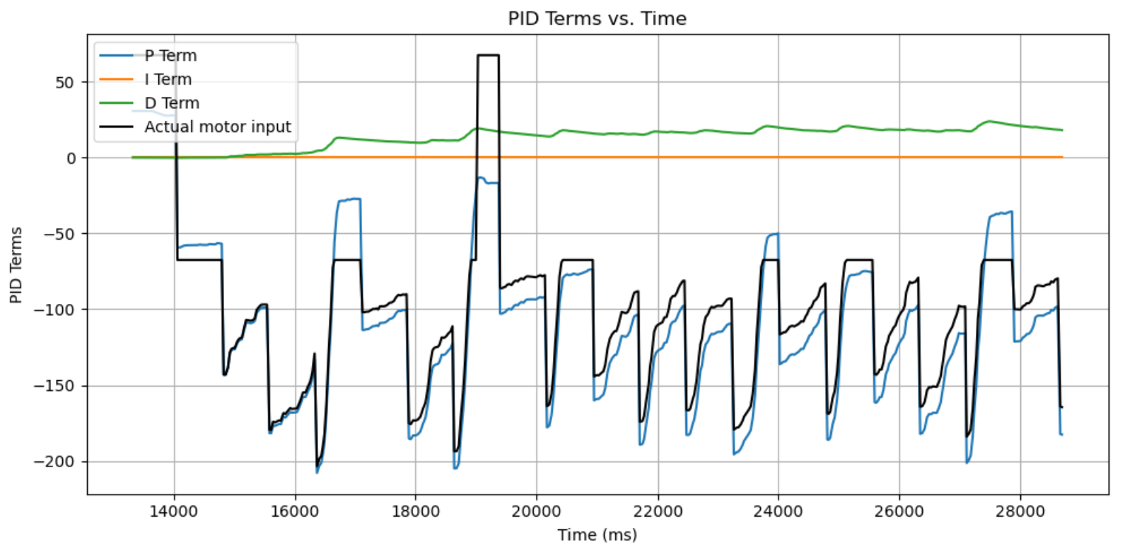
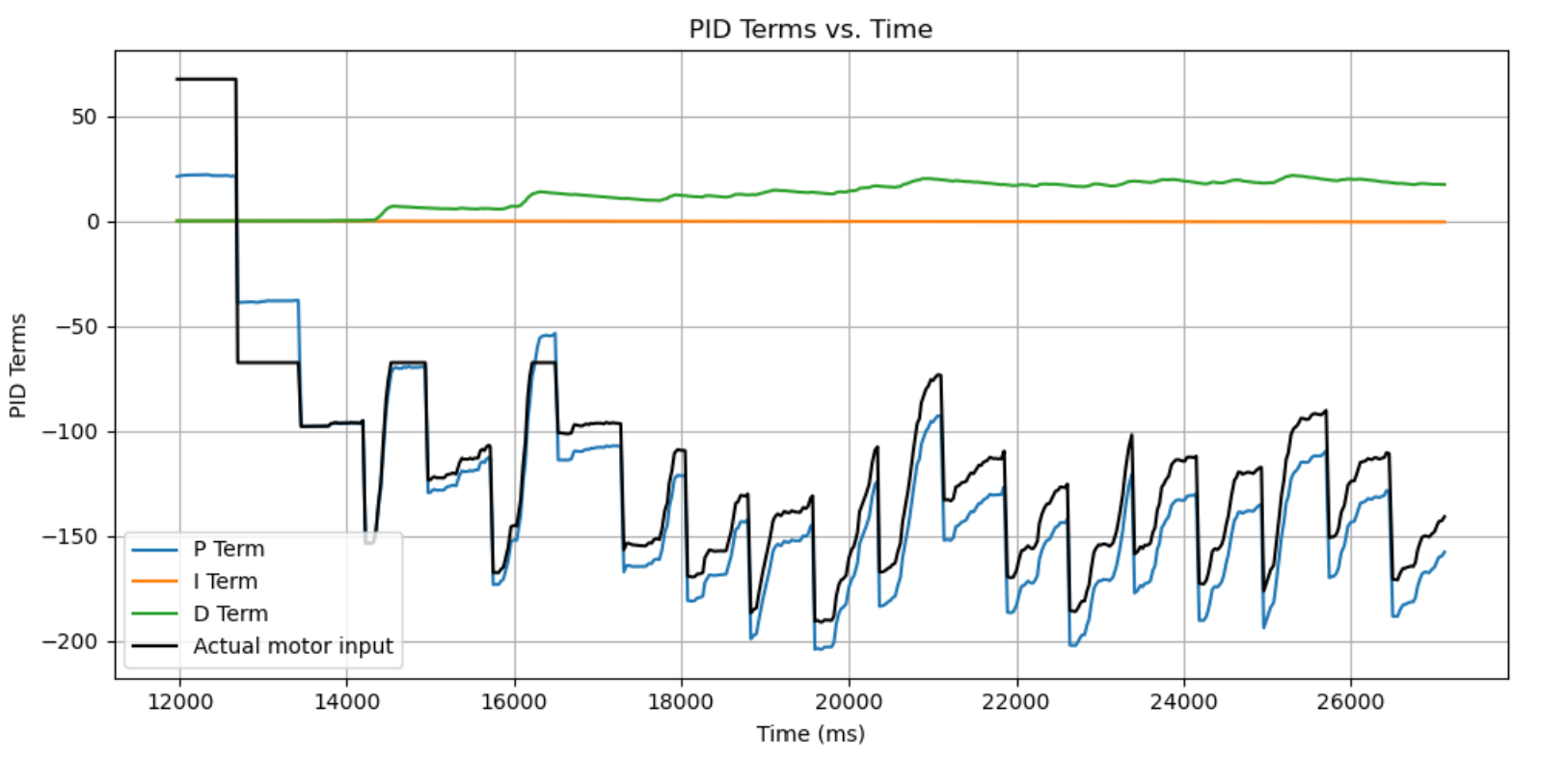
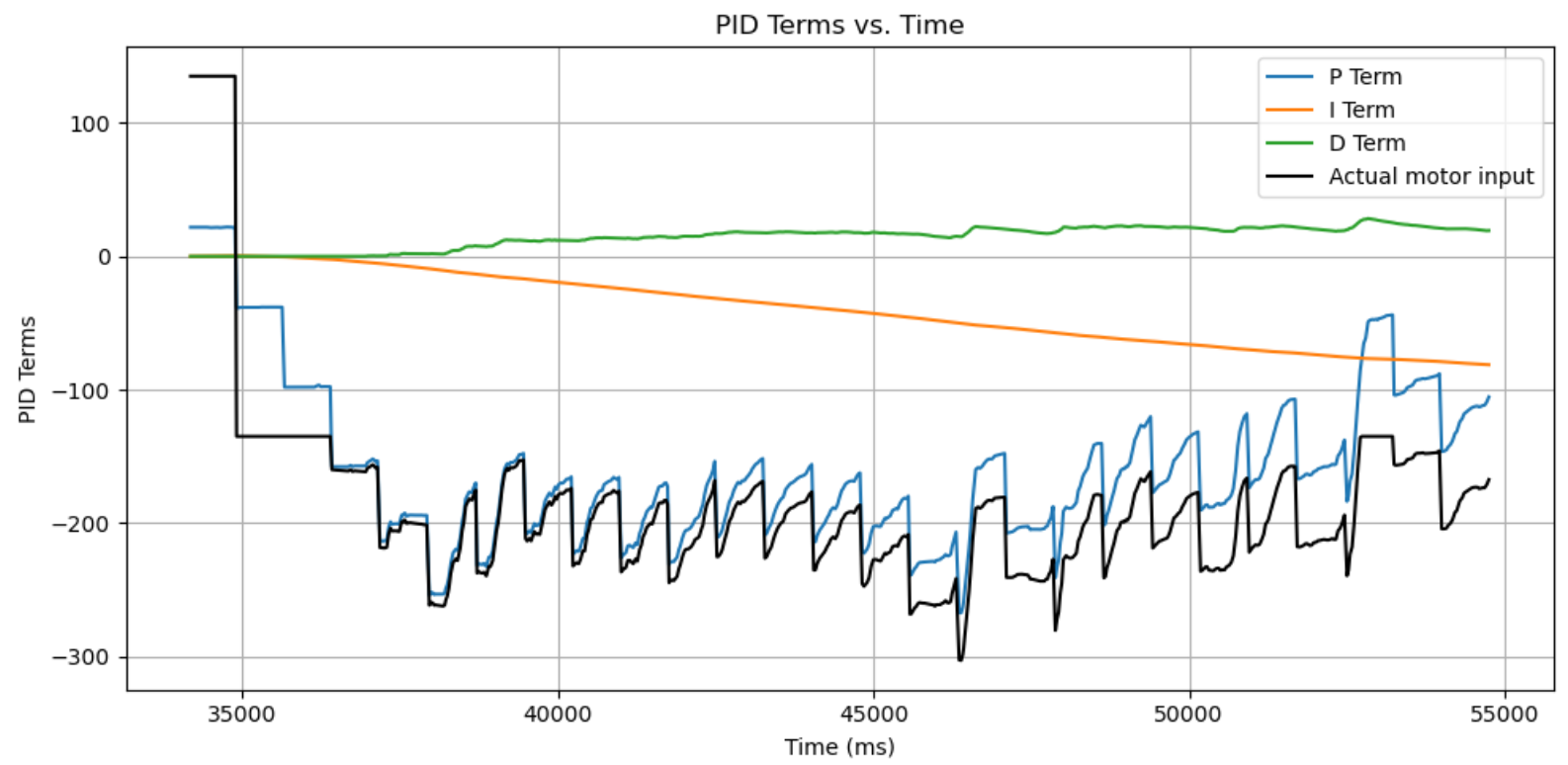
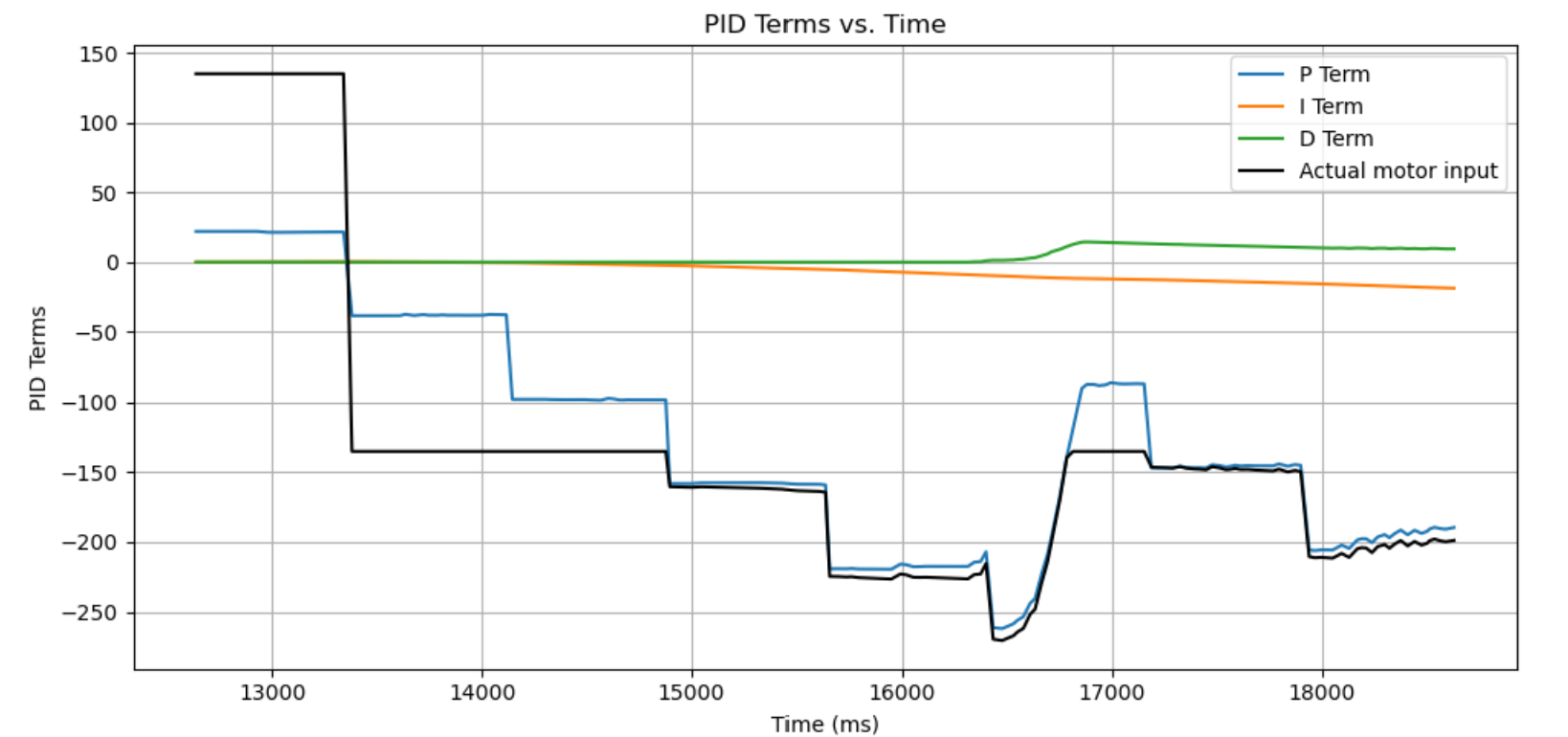
After some tuning, I realized that it may be best to use a PD controller because the timeframe that the robot stops for is too short for an integral term to contribute. So after some tuning, I got the robot to spin mostly on an axis with Kp = 6, Kd = 2, shown below.
To make sure that the PID control was working, I took the PID data from the on-axis test:
Discussion of Error
With the use of so many sensors, it’s important to discuss the potential errors arising from each one to understand how much error we should expect to see on our map.
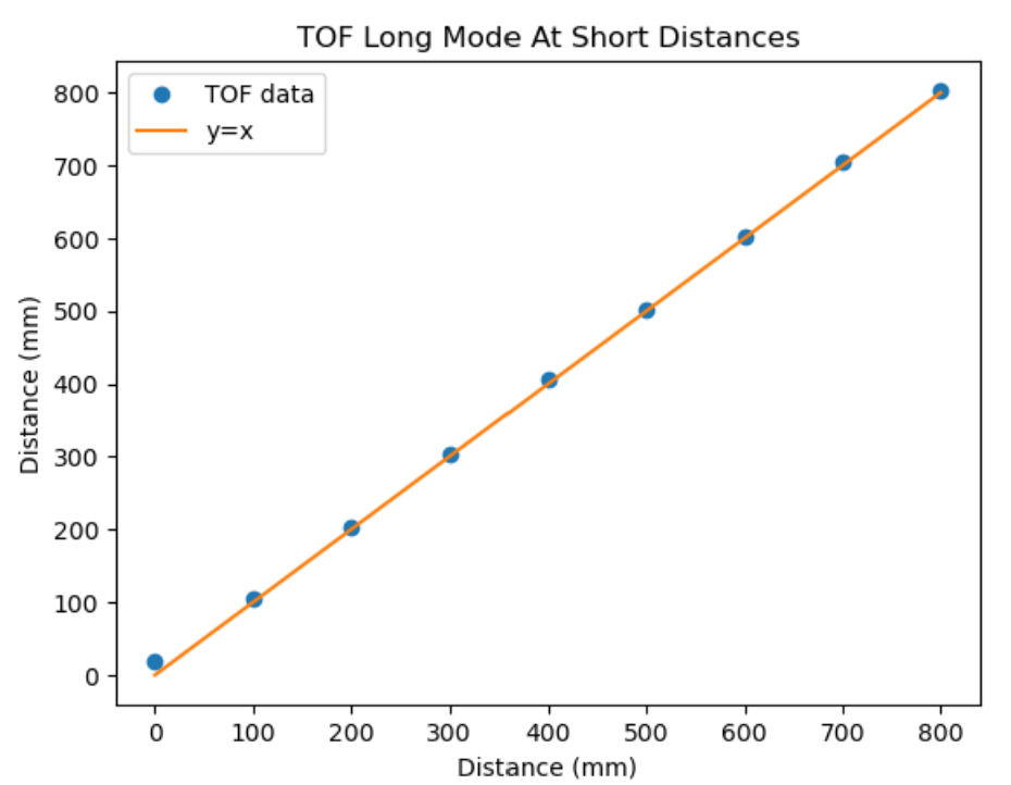
For the TOF sensor, I was mostly worried about the TOF’s accuracy at short ranges because I am using long mode for this lab. When I tested short mode in Lab 3, I found that the TOF sensor was amazingly accurate within +-5 mm within its documented range, so I was convinced enough that the error would be negligible at long distances since our grid is discretized to 1 ft = 304 mm. I did the same procedure as in Lab 3, holding up a ruler/making marks on the table at fixed distances, then seeing what the TOF outputs. The testing data showed that there was a discrepancy of 20 mm, but only at near-zero distances. This ends up being mostly negligible for our purposes because our testing locations are never that close to an obstacle.
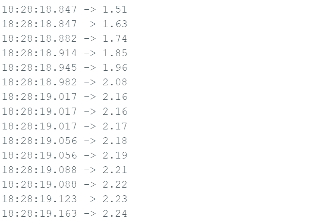
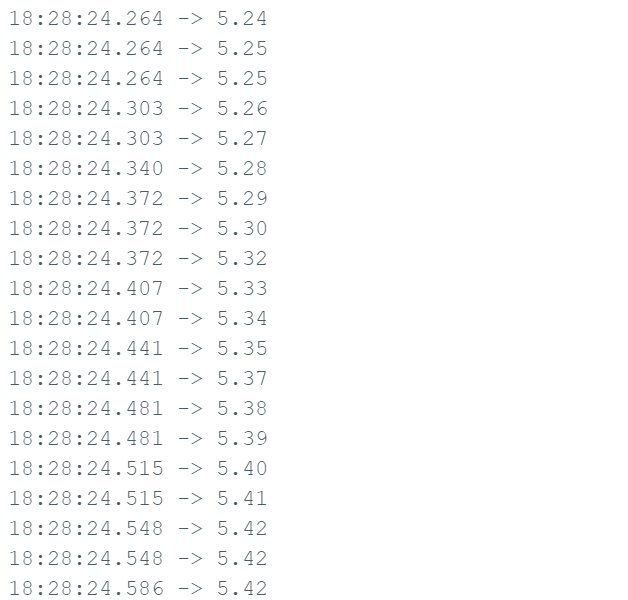
For the DMP, I wanted to see how much the sensor would drift, so I tested it by simply leaving the robot stationary and printing the DMP angles to serial. The results showed that the DMP would often start off and quickly drift to a small positive angle within a few seconds (5 seconds, in the test below). This poses an issue because during data collection I had told the robot to start immediately after I hit the reset button – this likely means a good chunk of data collection happened during this drift in angle. This likely caused the effect in the graphs below, where each dataset seemed to have their map shifted by a few degrees, making the resulting map tilted.
A final source of error is the inaccuracy of the on-axis turn. While the on-axis turn worked perfectly on some tiles, on other lab tiles the robot would slip. For the ones that did slip, there may be missing gaps in the data (although that is hard to quantify as an error numerically). And for other trials, I took the tape off of my robot. While that removed the slipping problem, the robot would sometimes drive to the end of the tile during its turn, meaning that measurements could be off by ~1 foot. It was also because of this that I neglected the translation from the robot-center frame to the TOF frame during my transformation matrix – since the location of the TOF does not really maintain constant and can’t be tracked precisely due to the variable movement and slipping during the turn, I thought it would be better to account for it in our error and post-process the results.
Summming up all of our potential errors we get that the maximum error is ~5 mm (TOF) + ~304 mm (robot movement) + ~76 mm (TOF translation) for distance ~= 385 mm. While the DMP angle is likely off by ~5 degrees. I don’t think I could quantify a distinct average error compared to maximum error because it seems like the sources of error are mostly constant (or rather they don’t really oscillate in any meaningfully predictable way). The DMP offset can be post-corrected during data processing, and the distance error (due to its inconsistency) gives us an explanation for seemingly incorrect data points.
Transformation Matrix
To do the transformation, I combined a translation with a rotation matrix. Since we have a point in the robot frame and want to convert it into the world frame, we know that x_world = R_robot->world * x_robot. To construct R, we think of a point measured by the TOF at heading theta. That point is at 0 degrees in the robot frame and at theta degrees in the world frame. So R must consist of a rotation by angle theta. The implementation of the function in python is given below.
def transform_robot_to_world(robot_pos, distance_array, angle_array_deg):
    """
    Transforms a set of sensor measurements from robot frame to world frame.

    Parameters:
    - robot_pos: tuple of (x, y) representing the robot's position in the world.
    - distance_array: array of distances measured by the TOF sensor, in mm.
    - angle_array_deg: array of absolute world orientation (yaw) angles in degrees.

    Returns:
    - Nx2 numpy array of (x, y) points in world coordinates.
    """
    # Convert angles from degrees to radians
    angle_rad = np.deg2rad(angle_array_deg)

    # Local robot coordinates (TOF is directly forward in robot x-direction)
    x_local = distance_array
    y_local = np.zeros_like(distance_array)

    # Create 2D rotation matrix for each angle and apply transformation
    world_points = []

    for i in range(len(distance_array)):
        theta = angle_rad[i]
        R = np.array([[np.cos(theta), -np.sin(theta)],
                      [np.sin(theta),  np.cos(theta)]])

        local_point = np.array([x_local[i], y_local[i]])
        world_point = R @ local_point + np.array(robot_pos)
        world_points.append(world_point)

    return np.array(world_points)
Implementing Mapping on Arduino
To do mapping on Arduino, I used a similar flow to Lab 8 because of the idea that we need to just complete one task. The data I need to fetch is also very similar to what I needed to get in Lab 6, so bluetooth functions already exist for sending the data back to the laptop. Now all I need to do is define a new bluetooth function to start the mapping task, which, in my implementation, also defines the angular PID gains. I’ve factored out the main logic into a separate function mappingSequence() for better readability.
case START_MAPPING:
{
  // Read gain inputs
  float kp_val, ki_val, kd_val;
  bool success_kp = robot_cmd.get_next_value(kp_val);
  bool success_ki = robot_cmd.get_next_value(ki_val);
  bool success_kd = robot_cmd.get_next_value(kd_val);

  if (success_kp && success_ki && success_kd){
    Serial.println("START MAPPING: Angle gains set successfully");
    angle_pid.setGains(kp_val, ki_val, kd_val);
  }
  else{
    Serial.println("Failed to set angle PID gains -- START_MAPPING");
  }

  // Reset global indices used for mapping
  mapping_index = 0;

  // Reset all of the data arrays used to store mapping (robot x, theta - will use normal timestamp_array w/ distance1 and angle_pid.meas_array)
  angle_pid.reset();
  angle_pid.setSetpoint(0.0); // should be 0 by default but just in case.
  for (int i = 0; i < array_size; i++){
    timestamp_array[i] = 0;
    distance1_array[i] = 0.0f;
  }

  // Call function defined in motors
  mappingSequence();

  // to be sure...
  stop();

  break;
}
The main function iterates through setpoint values in 15 degree increments and pauses for 750 ms at each point. Because of the non-dynamic nature of the task, I reasoned that it is okay to use delays until I get a new angle reading, effectively making the control loop the same frequency as the DMP values (~55 Hz). If we have TOF data, then we record the data point. The code is as follows:
void mappingSequence()
{
  // 10 deg. incr
  for (float sp = 0.0; sp < 391.; sp += 15.)
  {
    unsigned long startTime = millis();
    const int pauseTime = 750; // how long to stop at each setpoint
    angle_pid.setSetpoint(sp);

    // At each sp, we read angle and execute PID for [pauseTime] milliseconds.
    while (millis() - startTime <= pauseTime)
    {
      // We do not need to decouple rates of data vs. control loop, so we can use delays until we get data.
      float angle = getDmpYaw();
      while (!isValidYaw(angle))
      {
        delay(1);
        angle = getDmpYaw();
      }

      float d1 = getTof1IfReady();
      if (d1 != -1.0)
      {
        // Store angle and distance
        timestamp_array[mapping_index] = millis();
        angle_pid.meas_array[mapping_index] = angle;
        distance1_array[mapping_index] = d1;
        mapping_index++;
      }

      // Calc. PID & run
      int pwm = angle_pid.compute(angle);
      executeAnglePid(pwm);
    }
  }

  stop();
  return;
}
Raw Data
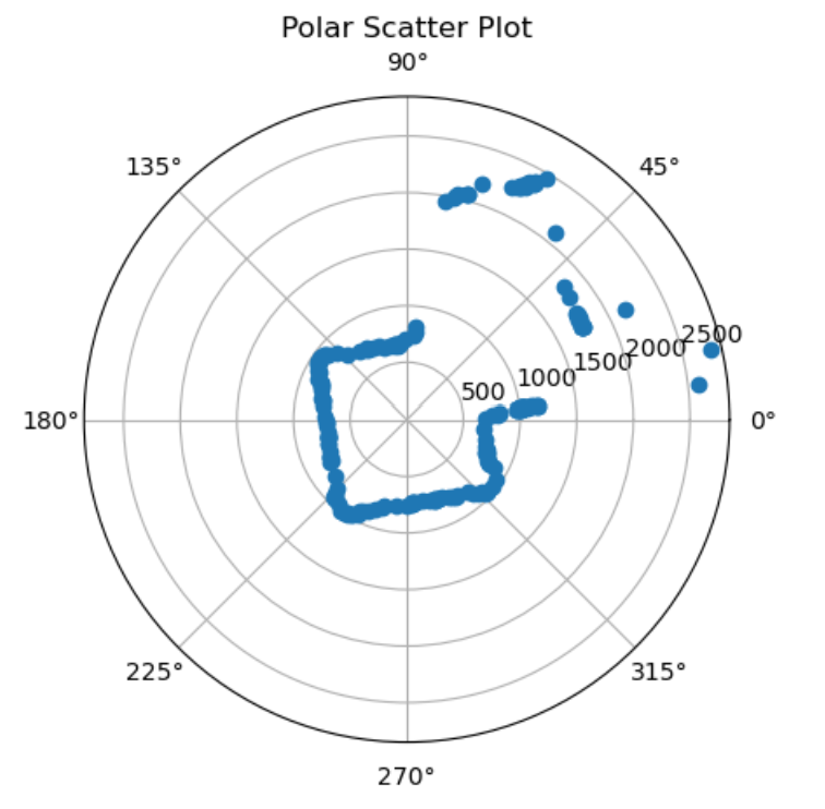
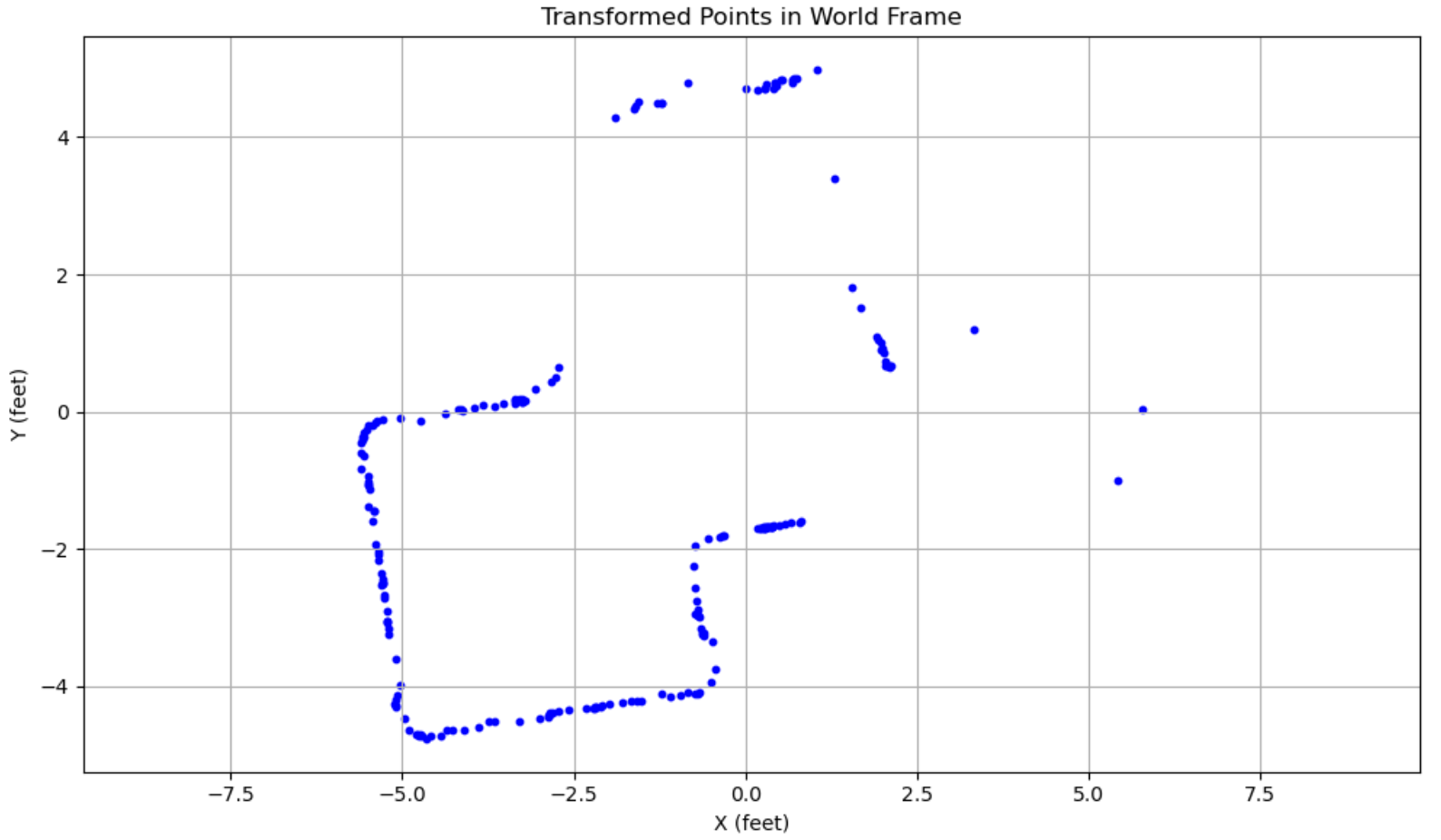
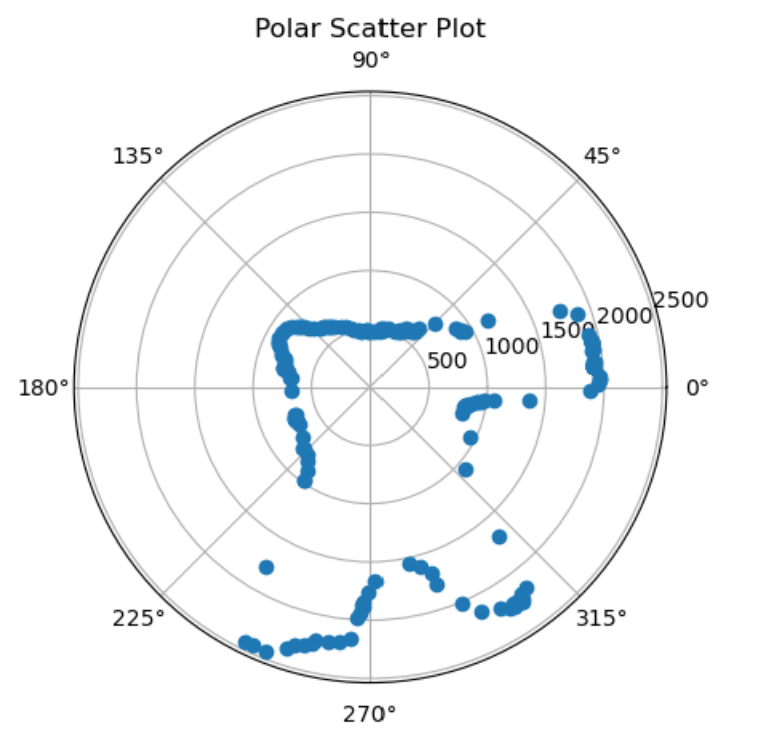
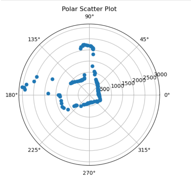
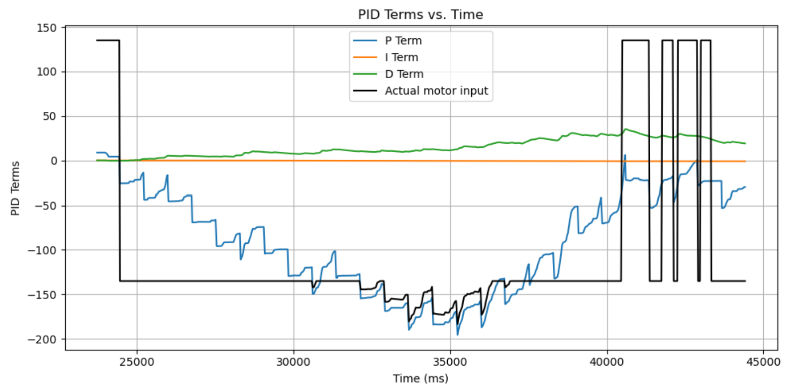
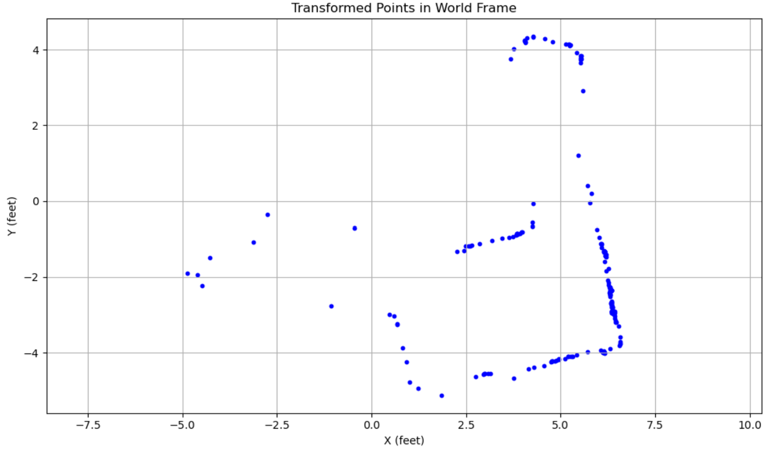
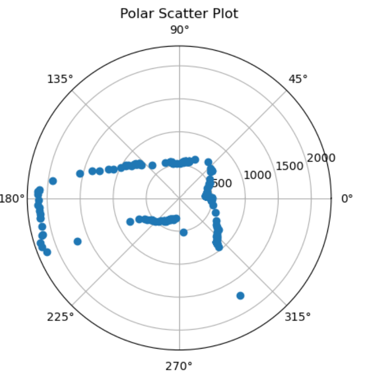
At each point, I collected the data to make a polar plot, a PID control plot, and the resulting transformed into global frame, just for a sanity check.
At point (-3, -2):
At point (0, 3):
At point (5, -3):
At point (5, 3):
Transformation to Global Frame
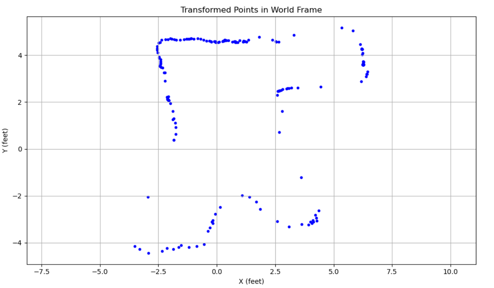
The raw globally transformed data into world frame (simply combining the four above) is as follows:
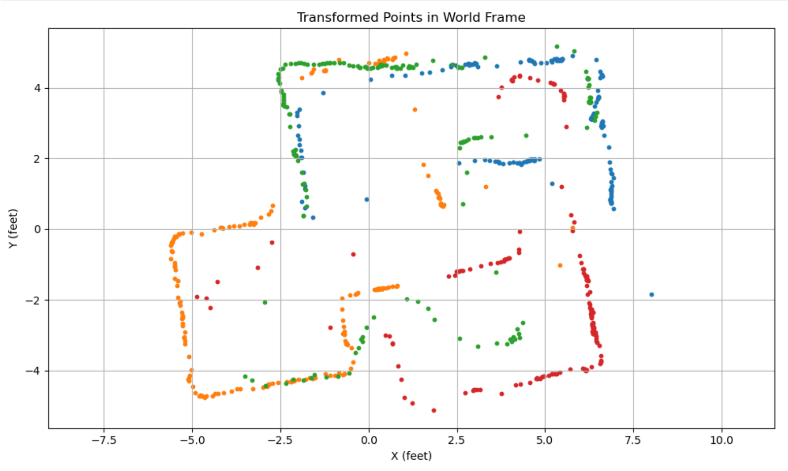
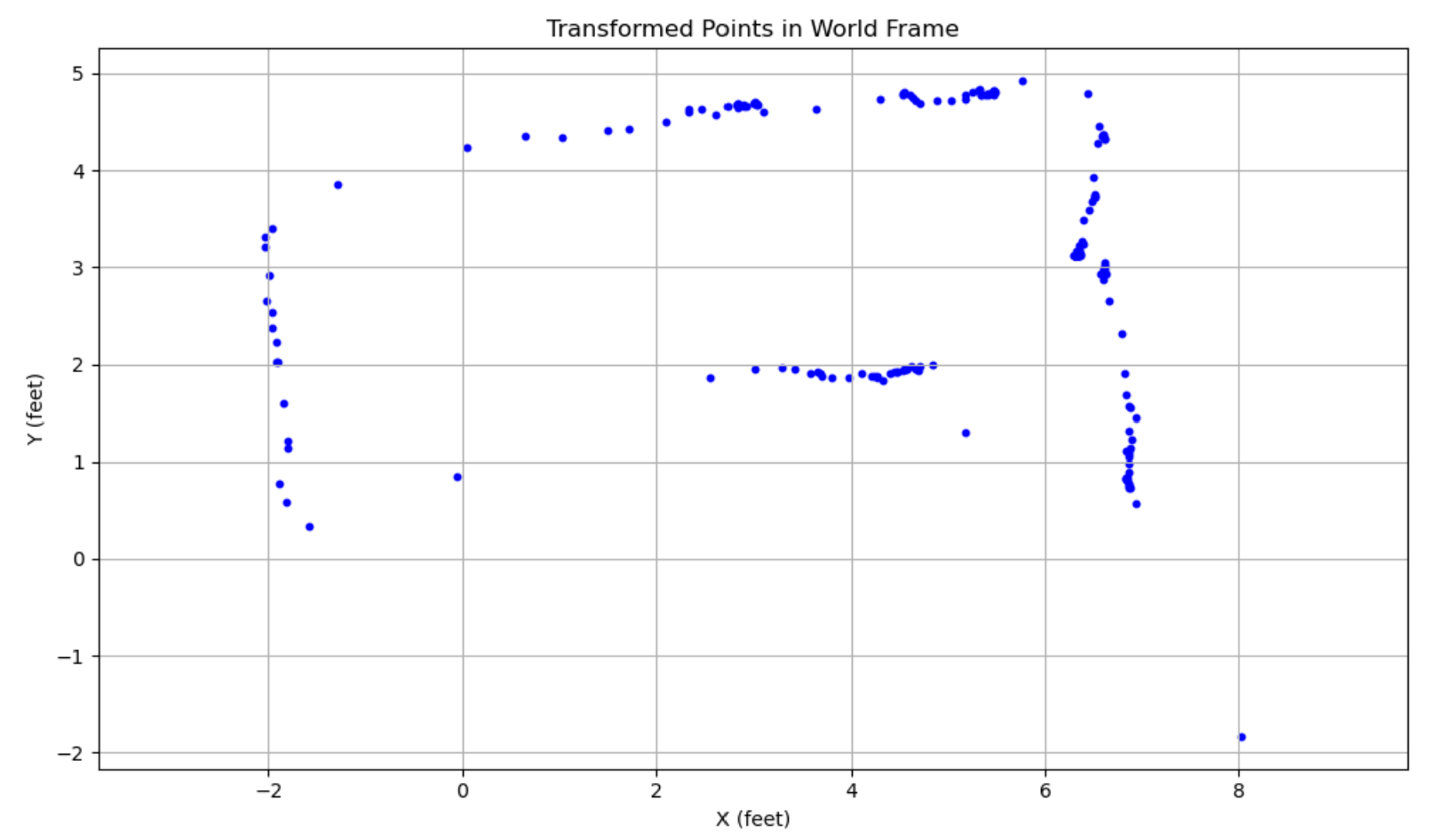
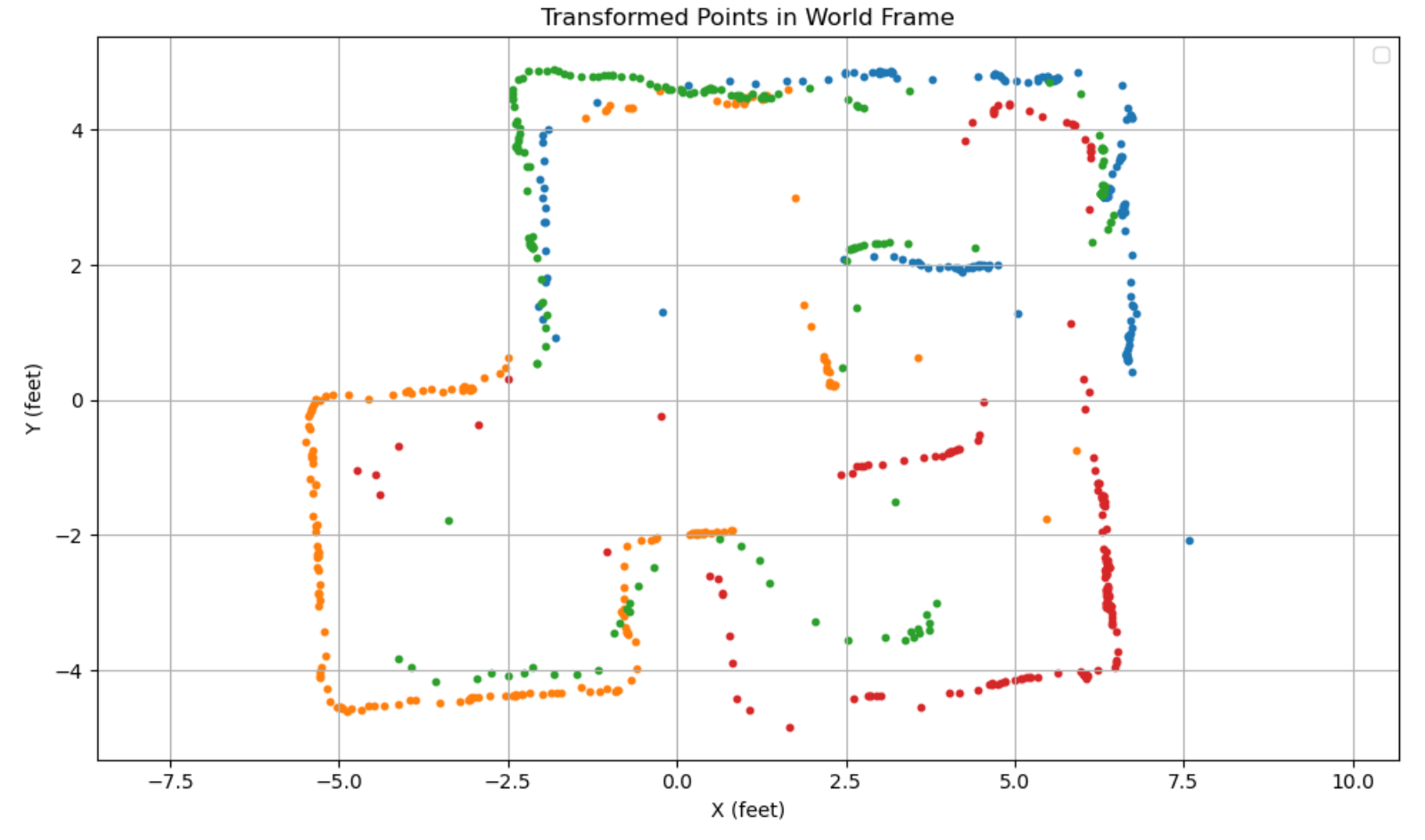
We can evidently see the effect of the DMP drift, since each subsection of the global graph seems to be tilted counterclockwise by a few degrees. This can be rectified by shifting the angle measurements in each section down by 5 degrees, which gives a straight rectilinear map like we expect:
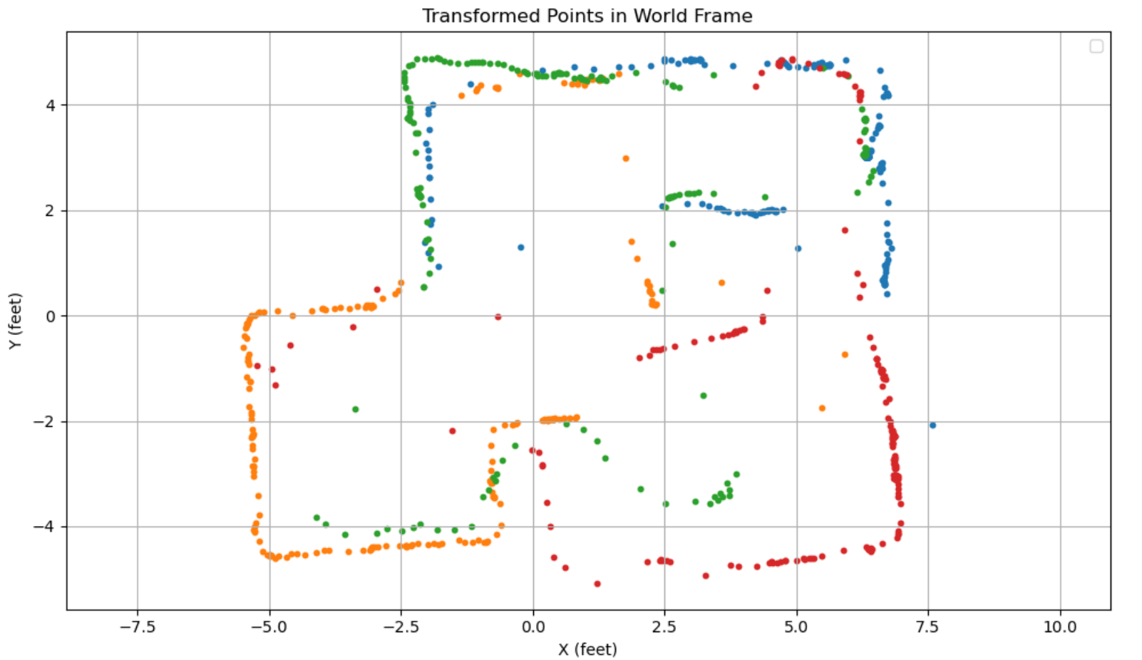
We can see the effects of our position error most clearly in the red at point (5, -3). It seems that all of the red points are shifted down by a half foot. This can also then be rectified in post, giving us a much nicer, final graph.
Drawing in Map Boundaries
With these points, we can draw in the rough map boundaries. Note that it seems like the orange and red datasets were angularly shifted by even more than the 5 degrees I rectified for, especially for the square boundary in the middle of our map. I mentally accounted for that fact by imagining the lines drawn by the orange and red to be rotated a few more degrees such that it closes the bounds drawn in black.
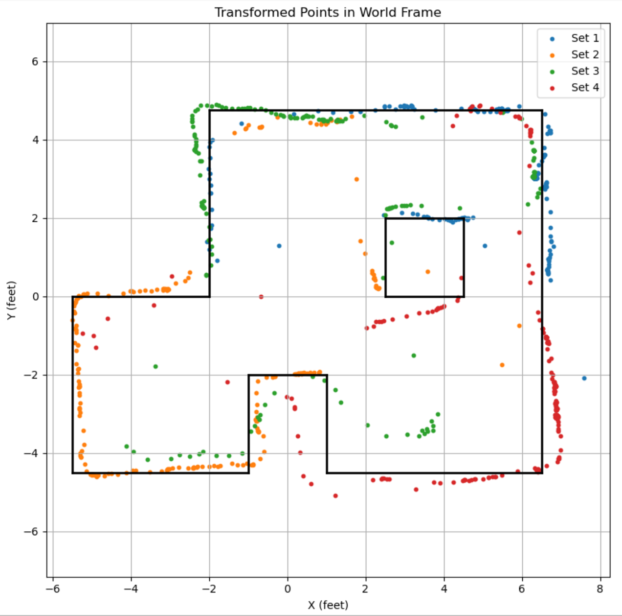
The set of endpoints used for my line segments is given as follows:
# Map line segments to plot
segments = [
    # boundary
    ((6.5, -4.5), (1, -4.5)),
    ((6.5, -4.5), (6.5, 4.75)),
    ((-2, 4.75), (6.5, 4.75)),
    ((-2, 4.75), (-2, 0)),
    ((-5.5, 0), (-2, 0)),
    ((-5.5, 0), (-5.5, -4.5)),
    ((-5.5, -4.5), (-1, -4.5)),
    ((-1, -4.5), (-1, -2)),
    ((-1, -2), (1, -2)),
    ((1, -2), (1, -4.5)),
    # square
    ((2.5, 2), (4.5, 2)),
    ((4.5, 0), (4.5, 2)),
    ((2.5, 0), (4.5, 0)),
    ((2.5, 0), (2.5, 2)),
]
Acknowledgements
- None specifically for this lab, but thanks to course staff for holding so many open hours so I could get this done!