Lab 7: Kalman Filter
Estimating Drag and Momentum
To find a state space representation of our system for the Kalman filter, we use a lumped mass-damper model and try to numerically estimate the drag and momentum terms. The equations we use to estimate drag and momentum terms are as follows:
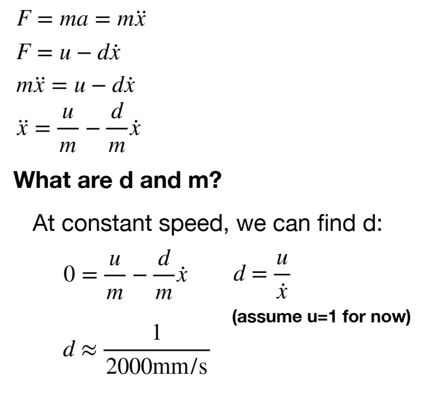
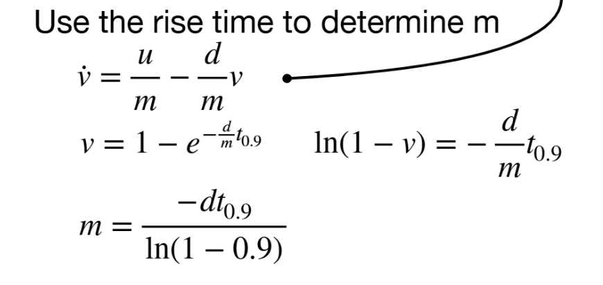
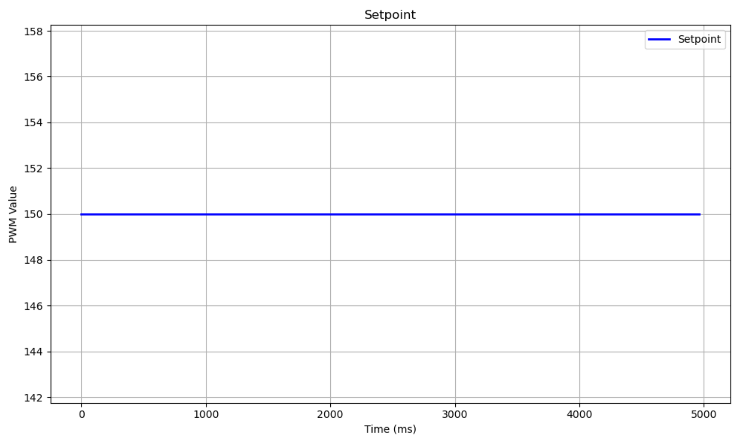
To do this, I ran the robot at a PWM strength on the higher end of what was used during linear PID, which was 150. This is in the desired range of 50-100% of maximum control input as well. A PWM of 150 was inputted the entire time, as shown below:
After getting the data, my first attempt was to fit an exponential decay curve onto velocity data. A fit is necessary compared to directly using the velocity values because the v data is naturally noisy due to having to use a finite difference between the TOF data points. The code snippet used and the result are as follows:
# Curve fit velocity
from scipy.optimize import curve_fit

# Define exponential model
def exp_decay(x, A, b):
    return A * (1 - np.exp(-b * x))

# Fit the curve
params, covariance = curve_fit(exp_decay, t, v, p0=(-3000, 1))

# # #
# In the plotting code we extend the t vector so we can see the forward
# projection of the exponential fit
# # #

# Compute fitted values
A_fit, b_fit = params
v_fit = exp_decay(t, A_fit, b_fit)

# Extend time values for fitted curve
t_extended = np.linspace(t[0], t[-1] + 1, 300)
v_fit_extended = exp_decay(t_extended, A_fit, b_fit)

# Plot original velocity vs. time
plt.figure(figsize=(10, 6))
plt.plot(t, v, 'o', label='Original velocity data', markersize=4)
plt.plot(t_extended, v_fit_extended, '-', label='Fitted exponential decay (extended)', linewidth=2)

#... more plot settings omitted
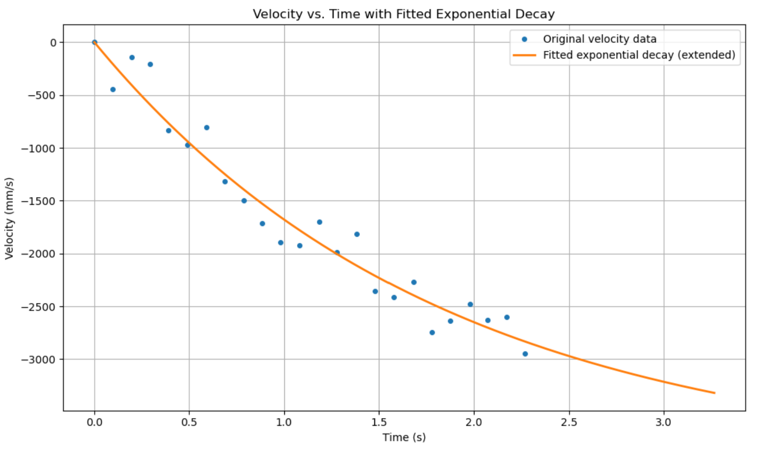
Evidently, the exponential fit generated insists that the plot is far from steady state, which is contrary to what I observed from lab. I ran the car across the outside lab room and into the hallway (which was the largest uninterrupted distance that I could find), and this was the largest continuous chunk of data I could get. Towards the end of the run pictured in the data, it didn’t seem like the car was accelerating at all. So, to confirm this and get a better sense of steady state velocity, I tried a secant-line fit on the last 2 data points of distance:
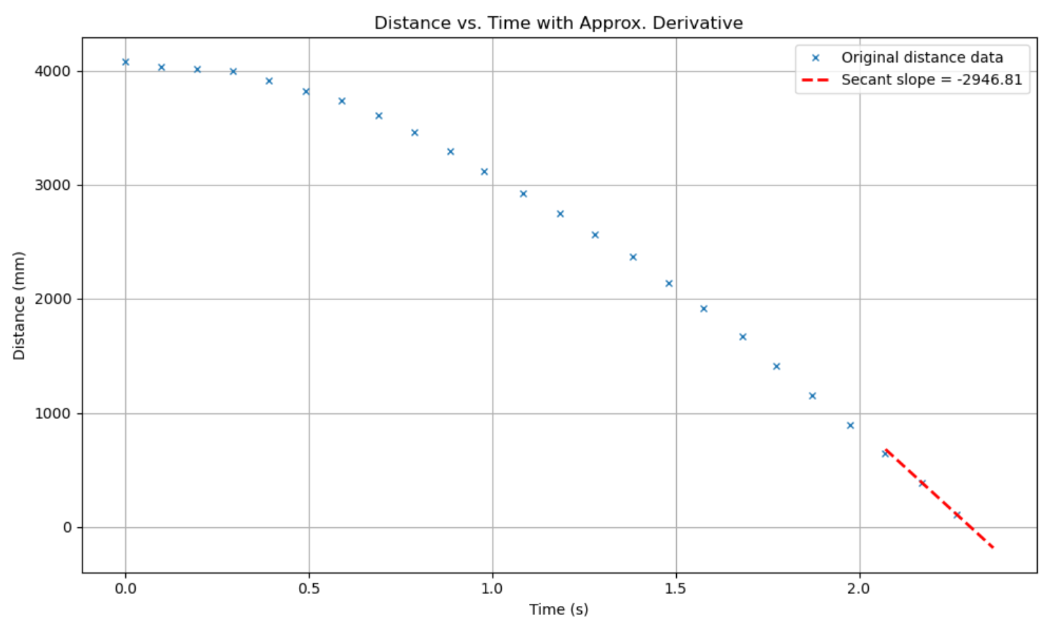
This gives me a steady state velocity of 2949 mm/s, which is far more in line with other values seen in other cars.
Thus, to estimate rise time, instead of using the curve fit, I will assume that steady state is exactly the value above, and approximate the point in time where the velocity graph reaches 90% of that value, or when it intersects v = 2654 mm/s.
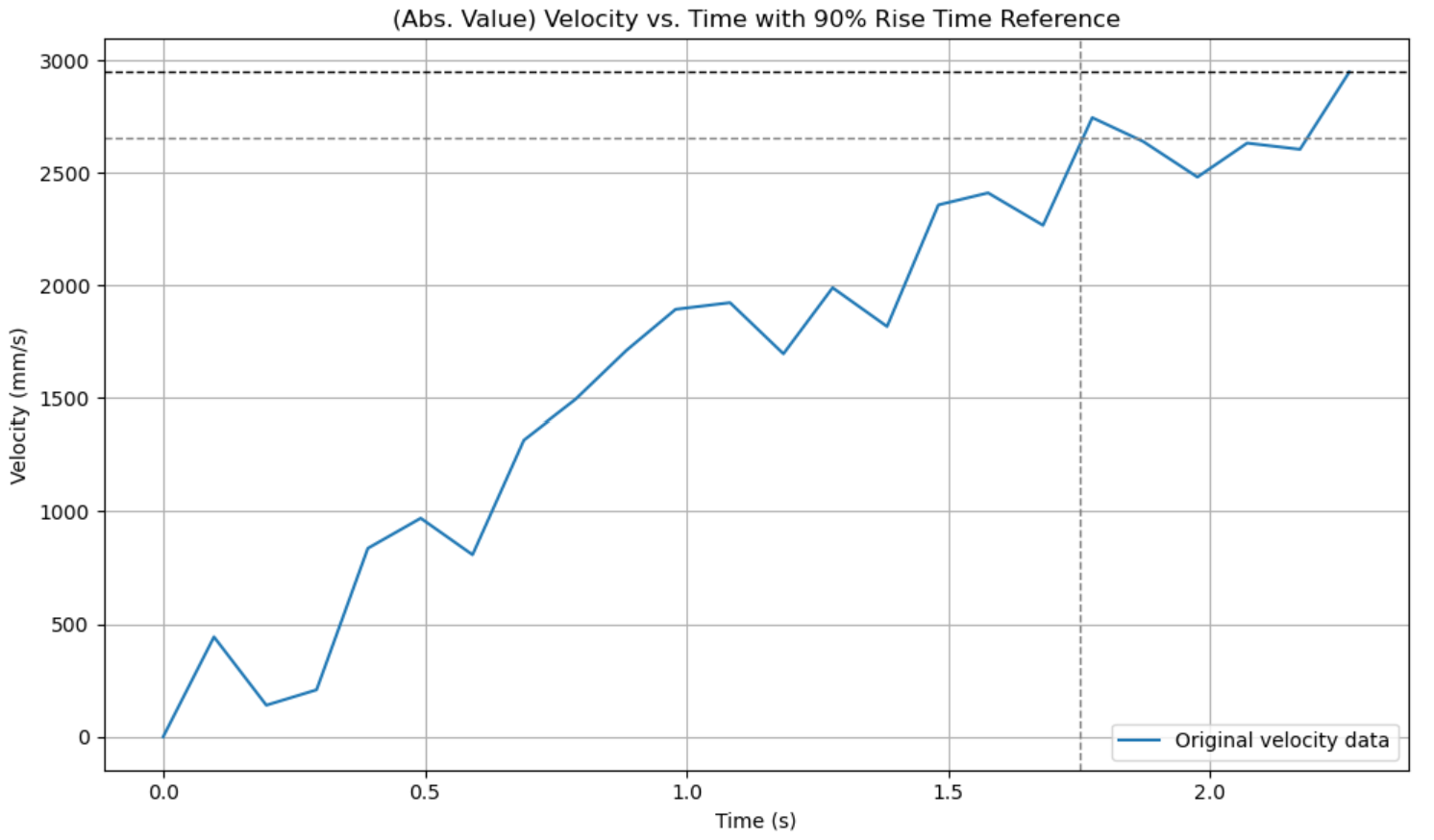
This shows that the 0-90 rise time was 1.752 s.
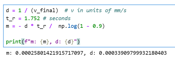
Combining these values, we get that d = 0.000339 and m = 0.000258. Note that we keep these values in millimeter-unit basis because the TOF sensor measures directly in millimeters. This way, we can get a better sense of what our variances physically mean.
Implementing Kalman Filter in Simulation
With our d and m values, we can initialize the A and B matrices according to our state space model. Our C is just going to be [1, 0] because we only want to measure the position.
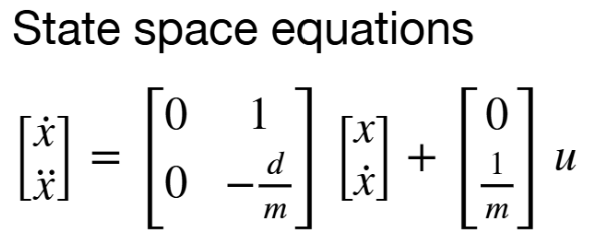
In Python, this is implemented with the code snippet:
dt = 0.1 #seconds, from TOF's 10 Hz

# State space construction where x_vec = [x; xdot]
A = np.array([[0, 1], [0, -d/m]])
B = np.array([[0], [1/m]])

# Discretized
Ad = np.eye(2) + dt * A  #2x2 identity
Bd = A * dt
C = np.array([[1, 0]]) # Measure just the distance
Our variance matrices are based off of sampling time, according to the lecture slides. I use my own sampling time calculated based on 10 Hz for sigma_1 and sigma_2, and used the recorded datasheet value on the slides, of 20 mm, for sigma_meas or sigma_3.
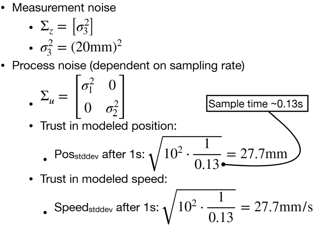
The code snippet is as follows:
# Sampling frequency
tof_freq = 10

# Process and measurement noise scalars
sigma_1 = np.sqrt(10**2 * tof_freq)
sigma_2 = np.sqrt(10**2 * tof_freq)
sigma_meas = 20

# Covar. matrices
sig_u = np.array([[sigma_1**2, 0], [0, sigma_2**2]])
sig_z = np.array([[sigma_meas**2]])

# Initial guess of covariance
sig_init = np.array([[20**2, 0], [0, 1**2]])
Then, we define the Kalman filtering code and call it on data I have from the positional PID lab:
# Load CSV file, skipping the header row
data = np.loadtxt('lab5_tof.csv', delimiter=',', skiprows=1)

# Separate into time and distance arrays
kf_test_time = data[:, 0]
kf_test_dist = data[:, 1]

kf_pred = []
x = np.array([[kf_test_dist[0]], [0]])
for i in range(len(kf_test_time)):
    x, sigma = kf(x, sigma, 1, kf_test_dist[i])
    kf_pred.append(x[0].item())

kf_pred = np.array(kf_pred)
This gives me the initial plot as follows:
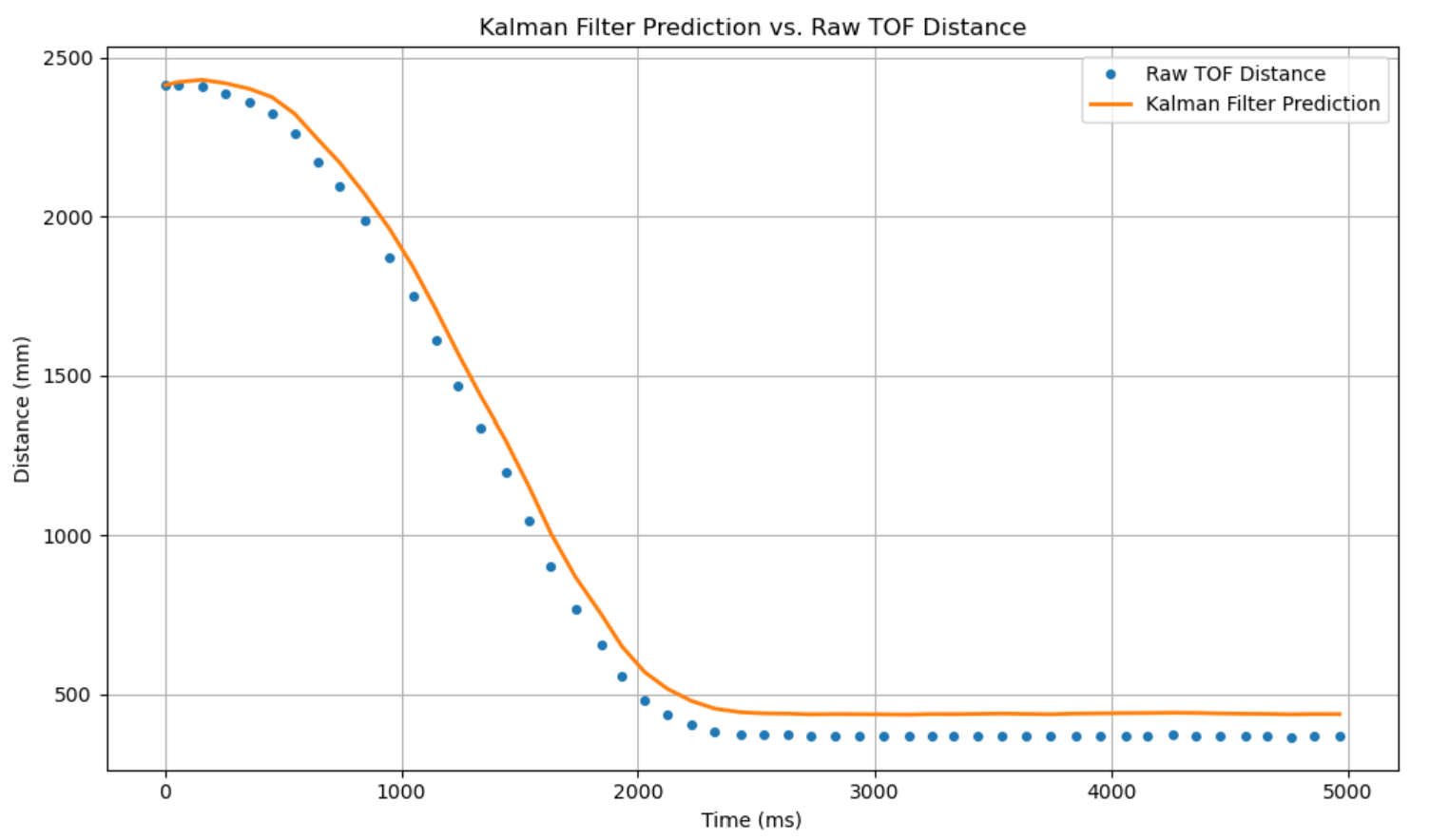
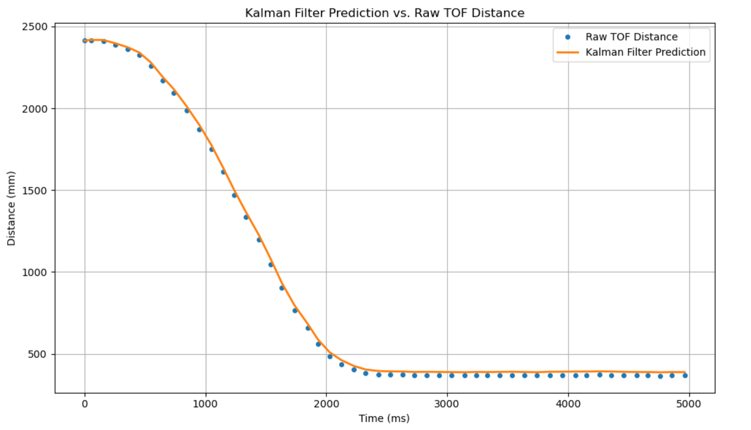
From this plot, I see that there is a lot of Kalman filter lag, meaning our system isn’t responsive enough. I don’t particularly want to modify the measurement noise since that is based off of an actual datasheet value. I noticed that the scalar of 10 in the sigma_1 and sigma_2 terms was more arbitrary than the sigma_3 term. By changing that scalar, I can increase the variances to position and velocity so that the Kalman filter is more susceptible to change.
With 20**2 instead of 10**2 in both sigma_1 and sigma_2, the KF fits the original data better.
Implementing KF in Arduino
Implementing the Kalman filter in Arduino involves storing the current belief of mean state and covariances, so I thought it would be best to encapsulate the functionality in a class. In a pair of files, the implementation is as follows:
kalman.hpp:
#ifndef KALMAN_FILTER_HPP
#define KALMAN_FILTER_HPP

#include <BasicLinearAlgebra.h>
using namespace BLA;

#include "config.hpp"

class KalmanFilter
{
public:
  // Constructor
  KalmanFilter(float dt, float mass, float dist, float sigma_meas, float sigma_proc_1, float sigma_proc_2);

  // Prediction step (called every control cycle)
  void predict(float controlInput);

  // Update step (called only when new measurement is available)
  void update(float measurement);

  // Getters
  float getPosition() const;
  float getVelocity() const;

  // Storage for KF data
  int kf_index;
  float position_array[pid_array_size];
  void initialize(float firstMeasurement); // Reset state + history

  // Normalizes PWM to be relative to u = 1.0 corr. to pwm 150.
  static float normalize(int pwm);

private:
  float dt_;
  Matrix<2, 2> A, Ad, sigma, sig_u, I;
  Matrix<2, 1> B, Bd, x;
  Matrix<1, 2> C;
  Matrix<1, 1> sig_z;
};

#endif
kalman.cpp:
#include "kalman.hpp"

KalmanFilter::KalmanFilter(float dt, float mass, float dist, float sigma_meas, float sigma_proc_1, float sigma_proc_2)
    : dt_(dt)
{
  // Continuous system
  A = {0, 1,
       0, -dist / mass};

  B = {0,
       1 / mass};

  // Identity matrix
  I = {1, 0,
       0, 1};

  // Measurement matrix
  C = {1, 0};

  // Discretized dynamics
  Ad = I + A * dt_;
  Bd = B * dt_;

  // Initial state
  x = {0, 0};

  // Initial covariance
  sigma = {400, 0,
           0, 1};

  // Process noise
  float q1 = sigma_proc_1 * sigma_proc_1;
  float q2 = sigma_proc_2 * sigma_proc_2;
  sig_u = {q1, 0,
           0, q2};

  // Measurement noise
  float r = sigma_meas * sigma_meas;
  sig_z = {r};

  // Clean measurement array
  for (int i = 0; i < pid_array_size; i++)
  {
    position_array[i] = 0.0f;
  }
}

void KalmanFilter::predict(float controlInput)
{
  Matrix<1, 1> u = {controlInput};
  x = Ad * x + Bd * u;
  sigma = Ad * sigma * ~Ad + sig_u;

  if (kf_index < pid_array_size)
  {
    position_array[kf_index] = x(0, 0); // log filtered position
    Serial.print("KF Pos:");
    Serial.print(x(0, 0));
    Serial.print(" | ");
    Serial.print("KF Velocity:");
    Serial.println(x(1,0));
    kf_index++;
  }
  else
  {
    Serial.println("KF array is full!");
  }
}

void KalmanFilter::update(float measurement)
{
  Matrix<1, 1> z = {measurement};
  Matrix<1, 1> S = C * sigma * ~C + sig_z;

  // Scalar inverse because S is 1x1
  Matrix<2, 1> K = sigma * ~C * (1.0f / S(0, 0));
  Matrix<1, 1> y = z - C * x;

  x = x + K * y;
  sigma = (I - K * C) * sigma;
}

void KalmanFilter::initialize(float firstMeasurement)
{
  x = {firstMeasurement, 0};
  //I trust position to be initially accurate to TOF's 5mm +-
  sigma = {25, 0, 0, 1};
  kf_index = 0;
  for (int i = 0; i < pid_array_size; i++)
  {
    position_array[i] = 0.0f;
  }
}

float KalmanFilter::normalize(int pwm)
{
  return (float)pwm / 150.;
}

float KalmanFilter::getPosition() const
{
  return x(0, 0);
}

float KalmanFilter::getVelocity() const
{
  return x(1, 0);
}
The initialization, in main, identically to in Python:
//KalmanFilter pos_kf(dt, mass, dist, sigma_meas, sigma_proc_1, sigma_proc_2);
// sigma_proc = sqrt(20^2 * 10) = 63.24
// sigma_proc = sqrt(10^2 * 10) = 31.62
// in mm units
KalmanFilter pos_kf(0.00856, 0.000258, 0.000339, 20, 63.24, 63.24);
I separated the update and predict steps so that I could decouple the TOF data rate with the control loop rate. In my main control loop, right before the motor drive function is called, I call the predict function. And every time valid data is obtained from the TOF, I call the update function. I omit that code because it could be placed in a variety of places with no different outcome.
One major point that Aidan pointed out was a sign disagreement between control input and the rate of change of my state. In my open loop test, I used 1.0 to correspond to a PWM of 150. Originally I had thought this means that any control input could simply be divided by 150.0. But in our state space equation, x double dot is dependent on positive 1/m * u, which means that a positive u would contribute positive x double dot, and therefore our x dot (in our case, the TOF reading), is increasing. Instead, because I chose my C matrix to be {1, 0} to observe position directly, I needed to negate my normalized control input so that a positive u causes a decrease in sensor measurement, as it is driving towards the wall.
A tiny code snippet from my motor drive functions, for illustration:
int input;
if (pwm > 0)
{
  // cast pwm to float for more accurate fp division?
  input = (int)clamp((float)pwm, DEADBAND, MAX_PWM);

  // Predict step every control
  // NOTE: a positive u suggests that distance is increasing, so we should negate u if it leads to decreasing dist.
  pos_kf.predict(KalmanFilter::normalize(-input)); // <------- NOTE THE NEGATION HERE

  drive(FORWARD, input);
}
// ... handle negatives, omitted
After implementing this, I now had an estimate of my position at all times, so I replaced any linear extrapolation calls and simply called pos_kf.getPosition() whenever I needed my current position.
PID Run With Kalman Filter
A run with Kp = 0.08, Ki = 0.002, and Kd = 0.02:
Graphs for position via Kalman filter and TOF are as follows:
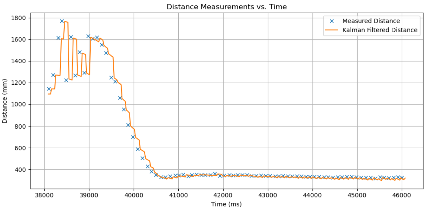
Some observations about the Kalman filtered position:
- It is able to follow the real TOF data readings with very little lag, indicating that our measurement noise term is not unreasonable.
- The velocity is hesitant to change rapidly, and conservatively estimates the velocity as it approaches the wall. Whether this is good entirely depends on the application of the robot. I would say it is acceptable for this class because the goal of this lab was to smoothly conduct a PID test, so there would be no sudden impulses in a typical run (unless it went extremely poorly).
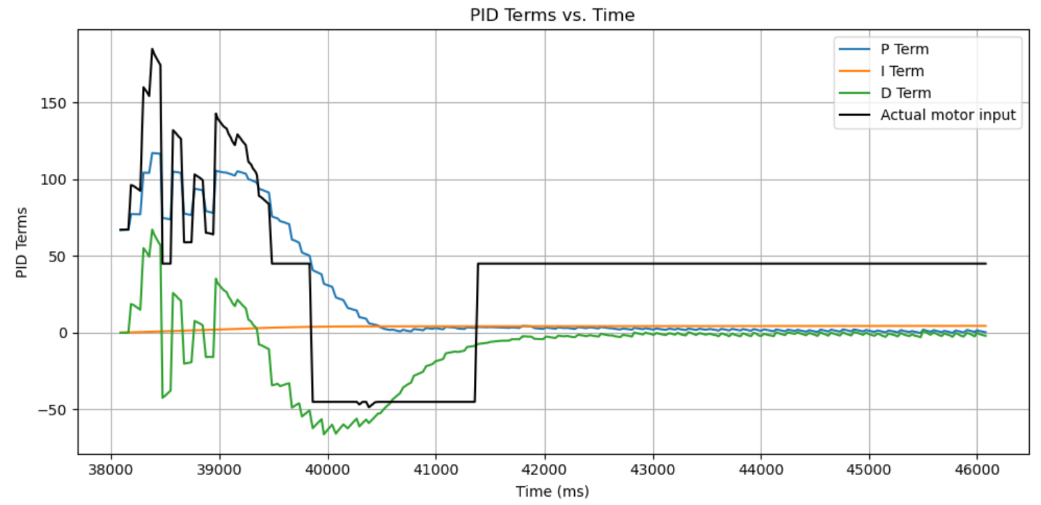
- The jumps from Kalman filter data to real TOF data doesn’t really cause a massive spike in my derivative control, so I am also satisfied with the ratio between the trust of our internal model compared to the trust of the sensor.
Finally, here is the PID control data, for completeness:
Acknowledgements
- Special thanks again to Aidan McNay for the life-saving advice on control input sign vs. C matrix sign!
- Thanks to Farrell for clarifying my questions on Ed so promptly!