Lab 5: Linear Distance PID
Prelab
For this prelab, I decided to use BLE to both change the gains and start the PID control loop. This is done by defining new BLE commands to be handled in Arduino. I added the following commands to the command types enum in Python, and its corresponding enum in Arduino (omitted):
class CMD(Enum):
  ...
  SET_KP = 5
  SET_KI = 6
  SET_KD = 7
  START_PID = 8
  STOP_PID = 9
  SEND_PID_DATA = 10
  PID_SPEED_TEST = 11
  PING_SPEED_TEST = 12
The SET commands are self explanatory, implemented by changing global variables. For example, SET_KP:
case SET_KP:
  {
    float val;
    success = robot_cmd.get_next_value(val);
    if (success)
    {
      Kp = val;
    }
    else
    {
      Serial.println("Setting Kp failed, KP NOT SET");
    }
    break;
  }
I also use a command to start up the PID so that I can upload code on my robot and have it be stationary until I want the controller to activate. The function sets a global flag to tell the robot to start doing PID, then resets all relevant data containers (which are also all global arrays):
case START_PID:
  {
    do_pid = true;
    pid_index = 0; //Sets return array index to 0.
    for (int i = 0; i < array_size; i++){
      timestamp_array[i] = 0;
      pwm_history[i] = 0;
      distance1_array[i] = 0.0;
    }
    pid_start_time = millis();
    break;
  }
The STOP_PID command is implemented, but I never used it so I will omit it here. Instead, there is an automatic hard stop implemented within the main function that executes every loop. If the time since pid_start_time exceeds a certain amount, the PID will be shut down:
void pidControlLoop()
{
  if (!do_pid) {
    brake(); // Similar to stop() in Lab 4 writeup, but writes all 255 instead of 0.
    return;
  }

  if (millis() - pid_start_time > 2000) {
    do_pid = false;
  }
  // ... GET TOF DATA AND DO CONTROL
}
Finally, the two other functions are used for gauging the main control loop speed vs. TOF speed. They will be discussed in the section below.
Speed of Control Loop vs. TOF
Once I structured my code to have a main control loop, I added the two last bluetooth commands to probe the speed of my TOF and control loop respectively. I first call the PID_SPEED_TEST command to start tallying the times the control loop is called, as well as whenever TOF data was ready. Then PING_SPEED_TEST sends the data in a string back to the computer.
case PID_SPEED_TEST:
  {
    doSpeedTest = true;
    testStartTime = millis();
    break;
  }
case PING_SPEED_TEST:
{
  tx_estring_value.clear();
  tx_estring_value.append("Main:");
  tx_estring_value.append(controlLoopCounter);
  tx_estring_value.append("|");
  tx_estring_value.append("TOF:");
  tx_estring_value.append(tofCounter);
  tx_characteristic_string.writeValue(tx_estring_value.c_str());
  break;
  }
The main loop for the speed test uses the same function that is used by the PID loop to see if the data is ready from the TOF sensor. This leverages the fact that the TOF sensor readings are always >= 0, which allows me to use -1.0 as a kind of null-value.
/*
* Returns: a float, the distance (in mm) recorded by TOF1 if the data is ready,
* Returns: -1.0 if the data is not ready.
*/
float getTof1IfReady()
{
  distanceSensor1.startRanging();
  int d1;
  if (distanceSensor1.checkForDataReady())
  {
    d1 = distanceSensor1.getDistance();
  }
  else
  {
    d1 = -1.0;
  }
  distanceSensor1.clearInterrupt();
  distanceSensor1.stopRanging();
  return d1;
}

...

void pidControlLoop()
{
  if (doSpeedTest){
    controlLoopCounter++;
    float d1 = getTof1IfReady();
    if (d1 != -1.0) tofCounter++;

    if (millis() - testStartTime > 2000){
      doSpeedTest = false;
    }
    return;
  }
  // ... REST OF PID LOOP CODE
}
This result of this test, conducted over 2 seconds, was recorded in Jupyter:
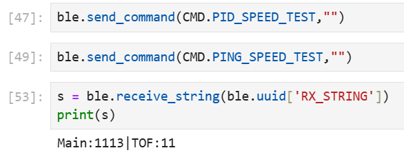
Note that this does slightly overestimate the frequency of the control loop, since the PID calculations were not done during this speed test. But I think this test encapsulates the main idea – that our control loop frequency far exceeds the TOF data frequency, and that decoupling the control logic from TOF reading was necessary.
PID Control
The code used to calculate the PID is fairly short. First, I define the global variables necessary for PID control:
#define MAX_PWM 100.0
#define MIN_PWM -100.0

// GOAL
float setpoint = 304; //mm

float PID_dt = 0.02; // s, default value
float Kp = 0.0;
float Ki = 0.0;
float Kd = 0.0;

float Ki_acc = 0.0;
float Kd_prev = -1.0; // init as invalid TOF reading to discern first iter

//Indexing return arrays. Should be set to 0 every time PID starts, in handle_command().
int pid_index = 0;

//Init automatically as zero. PWM and dist should never read zero: PWM we will add deadband to, and dist==0 indicates collision (bad!)
int pwm_history[array_size];
float pid_dist_history[array_size];

bool do_pid = false;
unsigned long pid_start_time = 0;
unsigned long pid_prev_time = 0;
A few things to note are that MAX_PWM and MIN_PWM are set so that I can first begin to start testing PID slowly. The index pid_index is incremented every time data is recorded, so the last data point can always be found at the index pid_index - 1. This creates a systematic way for me to access previous data points later, for linear extrapolation.
Then, the code to calculate the PID value directly follows from the formula. In my code, I broke the calculation into the constituent P, I, and D components then summed:
//Since goal is close to wall: let min pwm be more negative so that we can backpedal quickly
//Otherwise set relatively slow values...
#define MIN_PWM -150.0
#define MAX_PWM 100.0

// Helper function to keep values in range [low, high].
float clamp(float val, float low, float high)
{
  if (val > high){
    return high;
  }
  else if (val < low){
    return low;
  }
  else{
    return val;
  }
}

int calculatePID(float pos, float set)
{
  float error = pos - set;
  unsigned long cur_time = micros();

  if (pid_prev_time != 0){
    pid_dt = (cur_time - pid_prev_time) / 1000000.0; //sec
  }
  pid_prev_time = cur_time;

  Ki_acc += error * pid_dt;

  float derivative;

  if (Kd_prev != -1.000000000)
  {
    // NOT the first iteration -- proceed as normal
    // Anti-derivative kick: replace dError/dt with -dInput/dt
    // May want to implement a low-pass filter for high-noise data if TOF is messy, because a jittery input means dInput/dt goes crazy.
    derivative = (pos - Kd_prev) / pid_dt;
  }
  else
  {
    // the first iteration -- skip Kd term.
    derivative = 0;
  }
  Kd_prev = pos; //Save input for -dInput/dt of next loop

  float p = Kp * error;
  float i = Ki * Ki_acc;
  float d = Kd * derivative;

  return (int) clamp(p + i + d, MIN_PWM, MAX_PWM);
}
I kept the method of calculating PID separated from my main loop and logic for ease of debugging. For this lab, I could have just assigned setpoint instead of taking in the argument set, but the code would be easily modifiable once we get to planners and setpoints need to change.
I also separated out the method that interprets the PWM output and calls the motor driver functions, which allows me to easily edit the behavior of the motors without changing the PID algorithm:
void executePID(int pwm)
{
  // Because we never get to an absolute zero, we want to stop if our control effort is low.
  // This is necessary because of our +DEADBAND logic..
  if (abs(pwm) < 5){
    stop();
  }

  if (pwm > 0) {
    drive(FORWARD, (int) clamp(pwm + DEADBAND, MIN_PWM, MAX_PWM));
  }
  // pwm <= 0
  else {
    drive(BACKWARD, -((int) clamp(pwm - DEADBAND, MIN_PWM, MAX_PWM)));
  }
}
This code has two major features. First, it adds a minimum PWM to the motor input according to the deadband value found in the last lab. This way, we can fine tune the PID over actual control effort, since our calculations at lower PWM magnitudes would actually cause meaningful changes for the motors. Without this logic, calculations that result in |PWM| < DEADBAND would cause no motion in the motor. Secondly, this code stops the motor if PWM falls below a very small threshold. This is done primarily to prevent motor burnout towards the end of a trial, where we are approximately on the setpoint and the motor would otherwise vibrate back and forth. But an added benefit is to ensure that small PWM outputs don’t get magnified by our +DEADBAND rule and cause a jerking oscillatory motion at the setpoint.
Finally, the main control loop that is called in the main Arduino loop() gets TOF data. When the data is not ready, we use the last data points, either by purely using the previous point or by linear interpolation. If the data is ready, just use the new data point:
void pidControlLoop()
{
  if (!do_pid) {
    brake();
    return;
  }

  // DO PID FOR 5 SECONDS
  if (millis() - pid_start_time > 5000) {
    do_pid = false;
  }

  // TOF returns -1.0 if NOT ready
  float d1 = getTof1IfReady();

  int pwm;

  // TOF data is ready: record fresh data
  if (d1 != -1.0)
  {
    if (indexOutOfBounds(pid_index)){
      Serial.println("ARRAY FULL! Cannot write to array. Continuing PID control.");
    }
    else {
      timestamp_array[pid_index] = millis();
      distance1_array[pid_index] = d1;
      pwm = calculatePID(d1, setpoint);
      pwm_history[pid_index] = pwm;
      pid_index++;
    }
  }
  else
  {
    //Use previous point
    // pwm = calculatePID(distance1_array[pid_index-1], setpoint);

    //Linear interpolation
    pwm = calculatePID(distance1_array[pid_index-1] + linearExtrapolate1(), setpoint);
  }
  executePID(pwm); //Bumps up by DEADBAND and clamps.
  return;
}
PID Parameters & Execution
For this experiment, I started my car at 8 feet (within the range of TOF’s long mode) and the goal was for the car to stop at 1 foot from the wall. These two boundaries are marked by the orange tape in the video.
To start, I tuned the Kp to first get my car moving towards the wall. I don’t predict being able to go full speed towards the wall, so I set the max pwm output to 100 above. Doing a rough calculation, we want to move full speed near the start, so (2438.4 mm - 304 mm) -> (100 PWM). This gives us a conversion factor of Kp ~= 0.05.
Upon running this setting alone, I observe that the car immediately runs into the wall.
Kp = 0.05:
So to fix this, I wanted to add a Kd term to slow the car on its approach against the wall. Adding this, I observe that we’re most of the way there, but have some steady state error.
Kp = 0.05, Kd = 0.02:
To fix this, I wanted to add I, but upon adding the tiniest integrator term, I observe that the PWM sent to the motor is too fast. Seeing this, I gave up on the integrator term because it looked like I could tweak my PD controller to finish my task. In future labs, when I have more time, I will investigate why the integrator is giving such large values.
Kp = 0.05, Kd = 0.02, Ki = 0.001:
Finally, I tweaked the Kp and Kd slightly until the result was good enough for me.
Kp = 0.055, Kd = 0.025:
Note that I tried different left-right wheel calibrations to make it go straight, but after numerous tests, dust began accumulating on the wheels and changing the direction of the car slightly in every which way. Sorry.
Graph of Data
I collected both TOF sensor data and PID controller data. Note that these had to be done on different time bases because the control loop runs so much faster than the TOF. My TOF array and return are defined above, and I appended the following to record my PID control.
First, adding the necessary global arrays to store this data.
// 15 * array_size, for safety
#define pid_array_size 2250

// Global variables
int pid_control_index = 0;
int pid_timestamp_array[pid_array_size];
float p_array[pid_array_size];
float i_array[pid_array_size];
float d_array[pid_array_size];
Then, in the command type enum and handle_command():
case SEND_PID_CONTROL_DATA:
  {
    //Sends all data from PID. Assumes that no other data was collected.
    for (int i=0; i<pid_array_size; i++){
      tx_estring_value.clear();
      tx_estring_value.append("T:");
      tx_estring_value.append(pid_timestamp_array[i]);
      tx_estring_value.append("|");
      tx_estring_value.append("P:");
      tx_estring_value.append(p_array[i]);
      tx_estring_value.append("|");
      tx_estring_value.append("I:");
      tx_estring_value.append(i_array[i]);
      tx_estring_value.append("|");
      tx_estring_value.append("D:");
      tx_estring_value.append(d_array[i]);
      tx_characteristic_string.writeValue(tx_estring_value.c_str());
    }
    break;
  }
After that, I could simply write to these arrays during my calculate_PID() function:
int calculatePID(float pos, float set)
{
  //...rest of code
  float p = Kp * error;
  float i = Ki * Ki_acc;
  float d = Kd * derivative;
  pid_timestamp_array[pid_control_index] = millis();
  p_array[pid_control_index] = p;
  i_array[pid_control_index] = i;
  d_array[pid_control_index] = d;
  pid_control_index++;
  //... rest of code
}
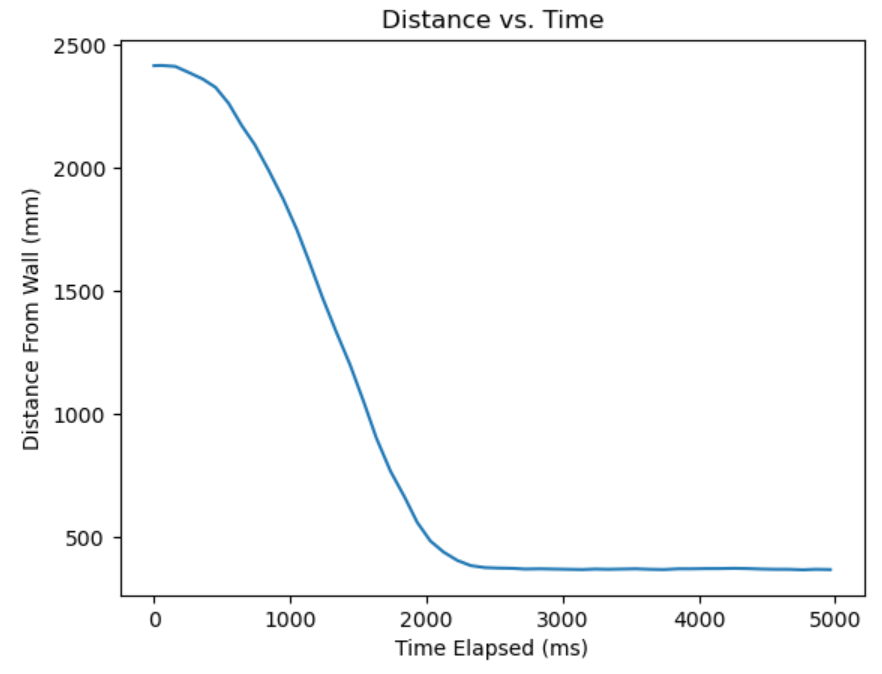
The TOF graph is relatively smooth:
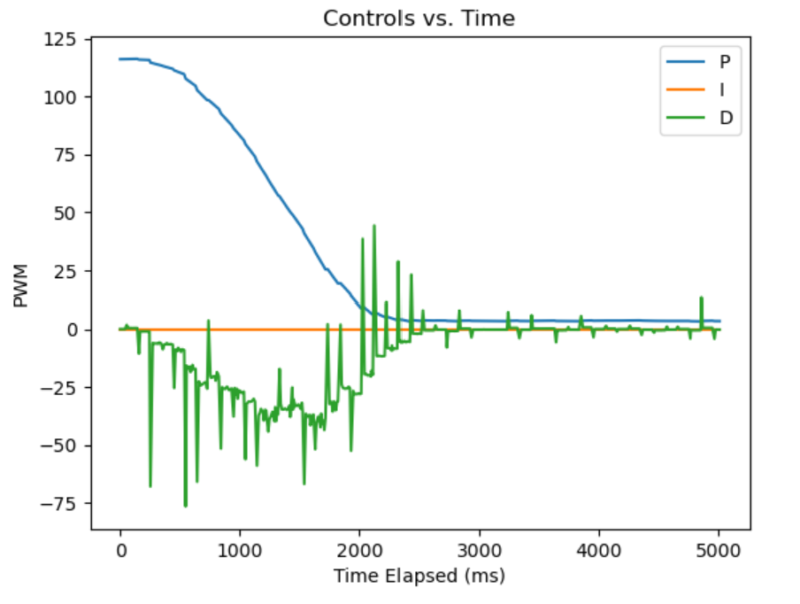
But the derivative term seems to have a huge amount of jitter. This is likely attributed to the fact that we use linear extrapolation until we get a new data point, but the velocity is not constant whatsoever during the execution. Every time a TOF update happens, we get a huge spike since the position we thought we were at was inaccurate.
References
- I asked my friends Sophia and Ben about how I should tune my PID gains.
- Additional shout out to Ben for helping me find two pesky negative signs in my PID expression. Turns out derivative control should not speed up into the wall!
- Also shout out to Adrienne for comic relief as always (don’t tell her I said that) 🫎.
- Thanks to Farrell for pointing out how my cross connector pins were sheared beyond belief.