Lab 3: Time Of Flight
Prelab
TOF Default I2C Address
According to the datasheet, section 1.1, the default I2C address is 0x52.
Method of Using Two TOFs
Since the two TOF sensors have the same default address, we need to change the address of one of them. To switch the address for a TOF sensor, we need to set XSHUT to a low state to disable one sensor while writing to the address of another. Then, we should set the XSHUT back so that both sensors are running and can be accessed via their unique addresses.
Placement of Sensors
I consulted robots of previous years, and realized that many students ended up using only one TOF’s data (in the front) for their main logic. Therefore, I will reserve one TOF for the front and one TOF for the back. During localization and mapping, this could create two points to cross reference. While a side sensor can serve a similar function, if any task requires driving backwards, the back TOF would be more useful than a TOF on the side. One potential downside, where collision may occur, is if we are driving near-parallel to a wall. Since our sensors are in the front and back, we could scrape against the wall and not be able to detect that we need to pull away.
Sketch of Wiring Diagram
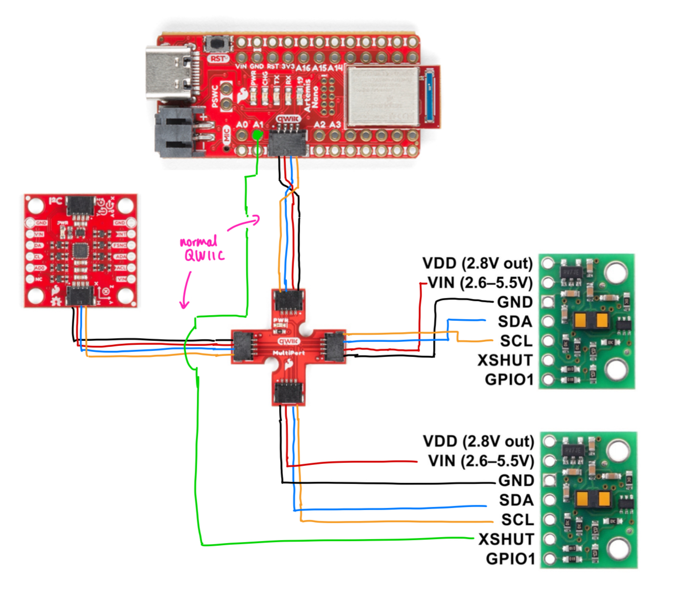
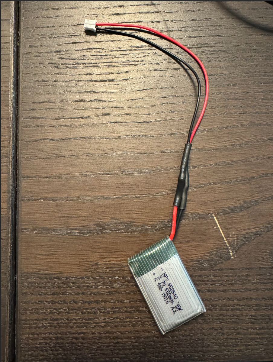
Connections & Powering the Artemis
To connect the Artemis to the battery, I cut and soldered my JST cable to the battery. Counterintuitively, the black wire on the JST plugs into the positive terminal on the Artemis. So, I soldered and heat-shrank the black lead to the positive battery end and red to negative.
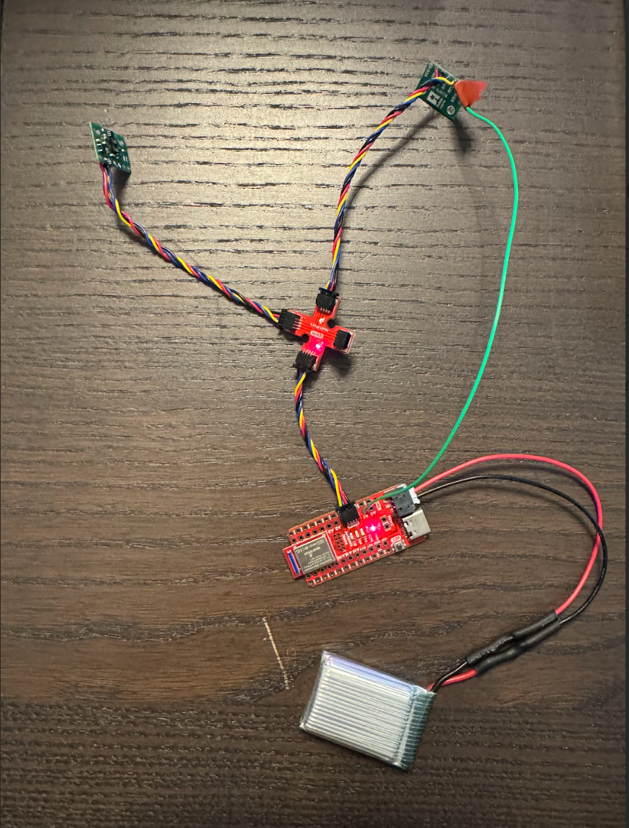
To demonstrate that the Artemis still functions without a wired connection, I tested some BLE code fetching IMU data from lab 2, which I know works because the array begins filling up:
The planned setup of the TOFs, Artemis, and IMU is as follows:
I2C Address
On running the example code found in Examples->Apollo3->Wire->Example05_Wire_I2C.ino, the Artemis returns the I2C address to be:
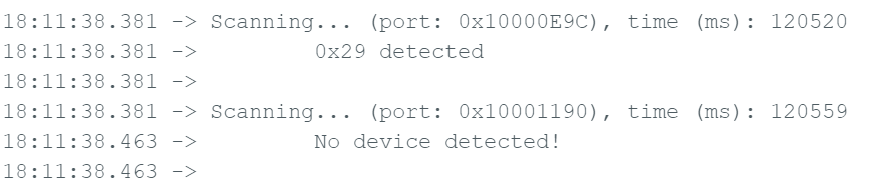
0x29 represented in binary is 0b101001. The datasheet indicated that the address was 0x52, which is 0b1010010 in binary. This means that the data sheet’s notation included the least significant bit in its representation, but Arduino ignores the LSB and returns 0x29 <=> (0x52 >> 1) because the LSB merely decides read vs. write.
One TOF Sensor & Testing
Short, Medium, Or Long
The TOF sensors have settinsg for short, medium, and long distance measurements. The documentation rates each mode for 1.3m, 3m, and 4m respectively. For most of the operation, I definitely want to run the TOF sensors in short mode because it gives us the best data granularity. The same resolution in bits recording a smaller number gives us a more precise distance reading. In practical operation, the robot should be able to adapt given that it senses an obstacle ~1.3 meters in front of it. Potentially the longer modes could be useful for making a rough map of the terrain, but I will definitely focus on testing the short mode.
Testing Short Mode
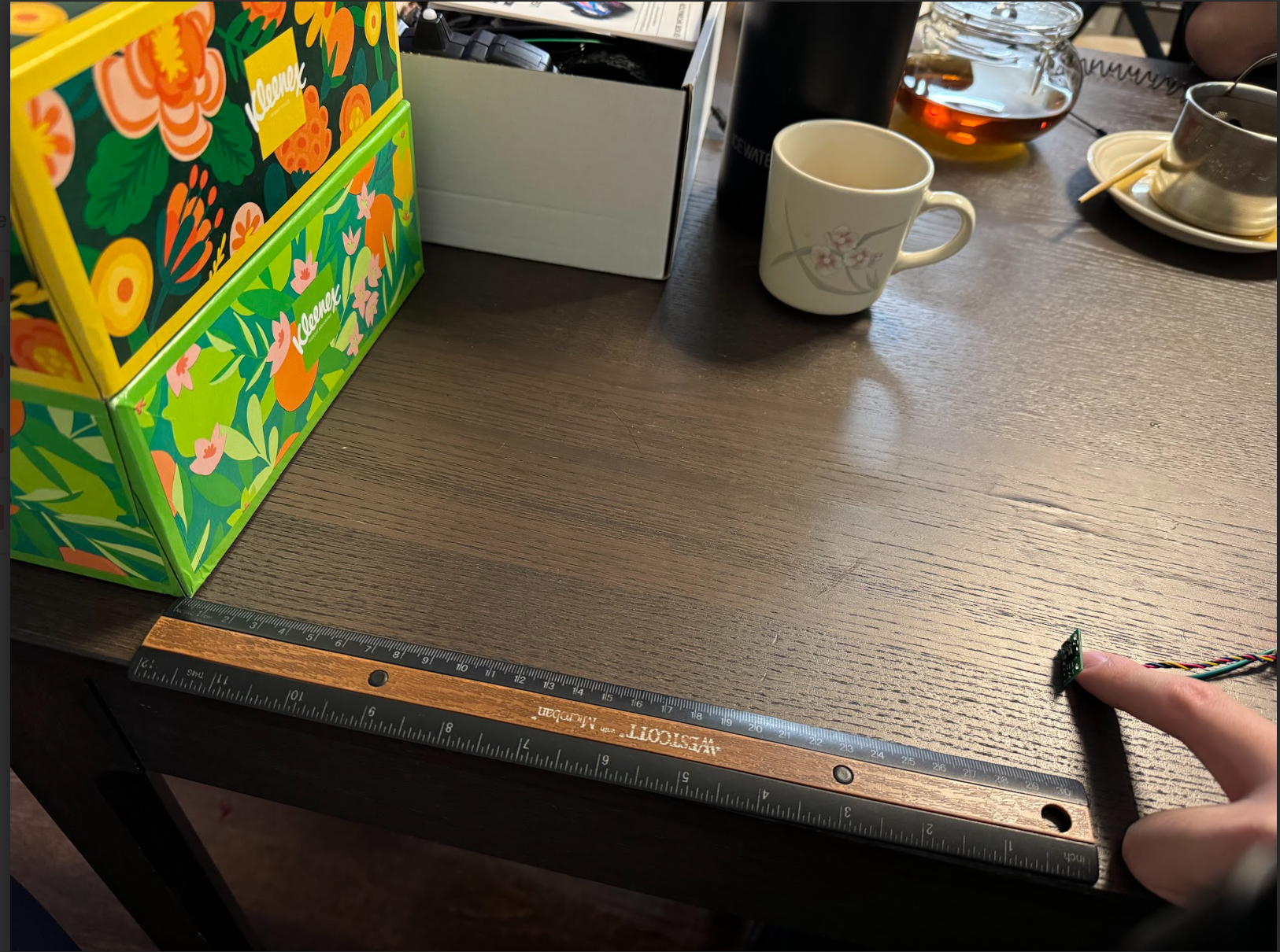
To test the TOF sensor independently, I set up an obstacle at the end of a long table, then placed a ruler, marking 10 cm intervals across the table. Then, I held the TOF at each marking, pointing it as directly at the obstacle as possible. At further distances, I made sure to lift it off the table so that the sensor would not hit the table rather than the obstacle.
At each distance, I used a BLE command to record 30 data points as quickly as possible, then transmitted it to Jupyter for processing. The code used modifies the example code from DistanceRead:
case GET_TOF_DATA:
  {
    distanceSensor.setDistanceModeShort();
    for (int i = 0; i < array_size; i++){

      distanceSensor.startRanging();  //Write config bytes

      while (!distanceSensor.checkForDataReady()){
        delay(1); //dubious
      }

      distance_array[i] = distanceSensor.getDistance();
      distanceSensor.clearInterrupt();
      distanceSensor.stopRanging();

      timestamp_array[i] = millis();
    }

    for (int j = 0; j < array_size; j++){
      tx_estring_value.clear();
      tx_estring_value.append("T:");
      tx_estring_value.append(timestamp_array[j]);
      tx_estring_value.append("|");
      tx_estring_value.append("D:");
      tx_estring_value.append(distance_array[j]);
      tx_characteristic_string.writeValue(tx_estring_value.c_str());
    }

    break;
  }
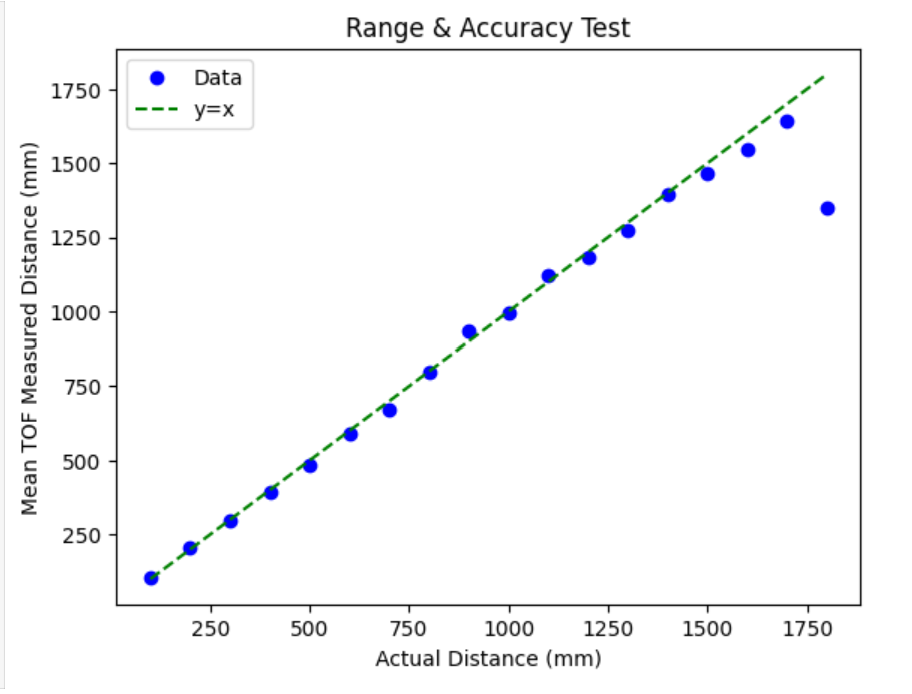
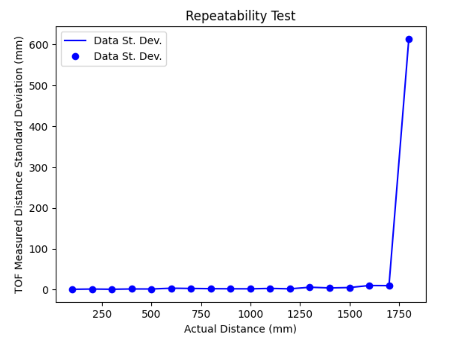
The accuracy and range can be seen by plotting the real distance to the TOF readings, and the repeatability can be visualized by plotting the standard deviation of the readings.
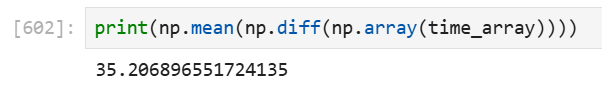
Since the data entries are taken as soon as possible, I can tell the ranging time by seeing the difference between the entries in the timestamp array. Note that this is only accurate to the millisecond because the timestamps are passed as ints. We can see that on average there is a delay of 35 ms between data points.
Thoughts on Short Mode
From the tests above, I concluded that the sensor was fairly accurate, usually within a couple millimeters, within its advertised 1.3 meter range. However, when the measured distance exceeded the 1.3 meter range, the accuracy drastically decreased. One possible error is that during testing, sometimes the TOF would produce drastically inaccurate results because I had not properly aligned the TOF to the obstacle I was pointing to. It would either hit the ground or miss the obstacle I was aiming at, causing large amounts of error. Therefore, when I assemble my robot, I will make sure to fix the TOFs firmly and not point them towards the ground, so large and unexpected errors don’t occur within the expected operating range.
Two TOFs
Setup
To utilize two TOF sensors at once, I controlled the XSHUT pin and altered the address of one of the TOFs to another valid I2C address. To test this easily, I created a new sketch with these components, then added the code to my larger BLE file afterwards.
At the top of the file, I import the library and define my pins:
#include <Wire.h>
#include "SparkFun_VL53L1X.h"

//Lab 3: TOF
//Optional interrupt and shutdown pins.
#define XSHUT 8 //In my wiring diagram I have pin 1, but I have since resoldered to 8 after it broke
#define ALT_I2C 0x30 //arbitrary within range 0x08 to 0x77; must be 7-bit valid

SFEVL53L1X distanceSensor1;
SFEVL53L1X distanceSensor2(Wire, XSHUT);
In setup(), I set XSHUT as a write pin and change the address of one of the TOFs:
Wire.begin();
Serial.begin(115200);
Serial.println("VL53L1X Qwiic Test (2 TOF)");

pinMode(XSHUT, OUTPUT); //write, to control XSHUT
distanceSensor1.setI2CAddress(ALT_I2C);
Serial.print("Address of TOF 1: 0x");
Serial.println(distanceSensor1.getI2CAddress(), HEX);

digitalWrite(XSHUT, HIGH); //disable TOF1
Serial.print("Address of TOF 2: 0x");
Serial.println(distanceSensor2.getI2CAddress(), HEX);
...
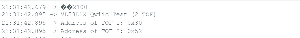
The output of the code indicates that the address was successfully changed:
Speed of Execution
In each loop, I print the current Artemis clock and continue if either data point is not ready:
void loop() {
  distanceSensor1.startRanging();
  distanceSensor2.startRanging();

  Serial.println(millis());
  if (!distanceSensor1.checkForDataReady() || !distanceSensor2.checkForDataReady()){
    return; //next loop if not ready
  }

  int d1 = distanceSensor1.getDistance();
  distanceSensor1.clearInterrupt();
  distanceSensor1.stopRanging();
  Serial.print("Distance1 (mm): ");
  Serial.print(d1);
  Serial.print(" | ");

  int d2 = distanceSensor2.getDistance();
  distanceSensor2.clearInterrupt();
  distanceSensor2.stopRanging();
  Serial.print("Distance2 (mm): ");
  Serial.println(d2);
}
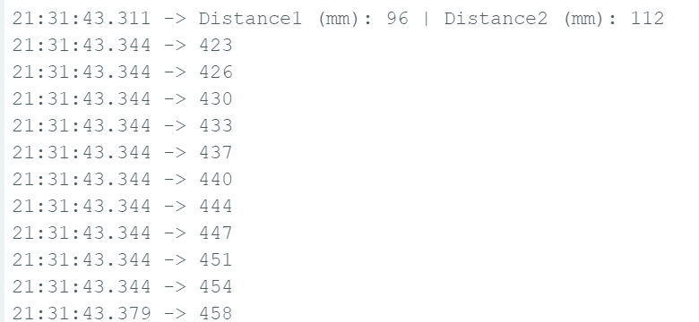
On average, the two-TOF data points were ready approximately every ~100 ms.
;
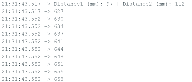
Clearly, the execution of the loop is much faster than the data can be collected for both TOF sensors. So the limiting factor is certainly the TOF sensor. To address this, I will need to make sure no code blocks on the TOF sensor readings, so that all components can run as fast as possible.
Measuring Two Distances
The following video executes code with the Artemis clock prints commented out. The two TOFs are pointed at the ceiling, approximately 1-2 meters above (it’s slanted). When I put a finger on each one, the corresponding output reads zero. All of this indicates that both sensors are working well.
Bluetooth
To send the data over Bluetooth concurrently with IMU, I adapted the code from Lab 2 and the one TOF case. First, I added GET_SENSOR_DATA as a command in cmd.py and on top of my Arduino file.
case GET_SENSOR_DATA:
{
  float complementary_pitch = 0, complementary_roll = 0; gyr_yaw = 0, dt = 0;
  gyr_last = micros();
  distanceSensor1.setDistanceModeShort();
  distanceSensor2.setDistanceModeShort();
  for (int i = 0; i < array_size; i++){

    distanceSensor1.startRanging();  //Write config bytes
    distanceSensor2.startRanging();  //Write config bytes

    while (!distanceSensor1.checkForDataReady()){
      delay(1); //dubious
    }
    while (!distanceSensor2.checkForDataReady()){
      delay(1);
    }
    distance1_array[i] = distanceSensor1.getDistance();
    distanceSensor1.clearInterrupt();
    distanceSensor1.stopRanging();

    distance2_array[i] = distanceSensor2.getDistance();
    distanceSensor2.clearInterrupt();
    distanceSensor2.stopRanging();

    if (myICM.dataReady())
    {
      myICM.getAGMT();
      float theta = atan2((&myICM)->accX(), (&myICM)->accZ())  * (180.0 / M_PI);
      float phi = atan2((&myICM)->accY(), (&myICM)->accZ()) * (180.0 / M_PI);
      dt = ( micros() - gyr_last) / 1000000.;
      gyr_last = micros();
      gyr_yaw = gyr_yaw + myICM.gyrZ()*dt;

      complementary_pitch = (complementary_pitch - myICM.gyrY()*dt)*(1-alpha_complementary) + theta * alpha_complementary; //also negate gyro
      complementary_roll = (complementary_roll + myICM.gyrX()*dt)*(1-alpha_complementary) + phi * alpha_complementary;

      complementary_roll_array[i] = complementary_roll;
      complementary_pitch_array[i] = complementary_pitch;
      gyr_yaw_array[i] = gyr_yaw;

    }
    timestamp_array[i] = (int) millis();
  }

  for (int j = 0; j < array_size; j++){
    tx_estring_value.clear();
    tx_estring_value.append("T:");
    tx_estring_value.append(timestamp_array[j]);
    tx_estring_value.append("|");
    tx_estring_value.append("D1:");
    tx_estring_value.append(distance1_array[j]);
    tx_estring_value.append("|");
    tx_estring_value.append("D2:");
    tx_estring_value.append(distance2_array[j]);
    tx_estring_value.append("|");
    tx_estring_value.append("Roll:");
    tx_estring_value.append(complementary_roll_array[j]);
    tx_estring_value.append("|");
    tx_estring_value.append("Pitch:");
    tx_estring_value.append(complementary_pitch_array[j]);
    tx_estring_value.append("|");
    tx_estring_value.append("Yaw:");
    tx_estring_value.append(gyr_yaw_array[j]);
    tx_characteristic_string.writeValue(tx_estring_value.c_str());
  }

  break;
}
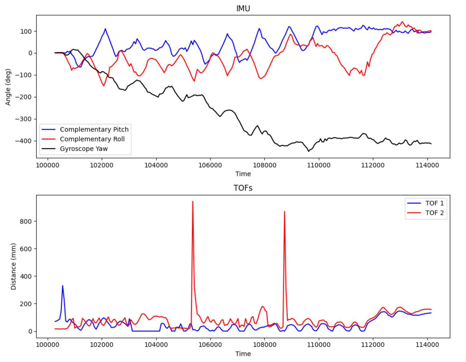
Using this code, I can verify that IMU data and TOF data is being collected simultaneously. Note that there is still the issue where gyroscope data only collects during Bluetooth command, and I am still investigating that. However, this shows that both types of sensors can be passed at the same time.
References
- I referred to Mikayla Lahr and Wenyi Fu’s websites as guides on the soldering connections. I also took some inspiration from how they set up their TOF, particularly when to use the XSHUT pin.
- This link clarifying how the XSHUT is pulled up to high by default.
Appendix: Jupyter
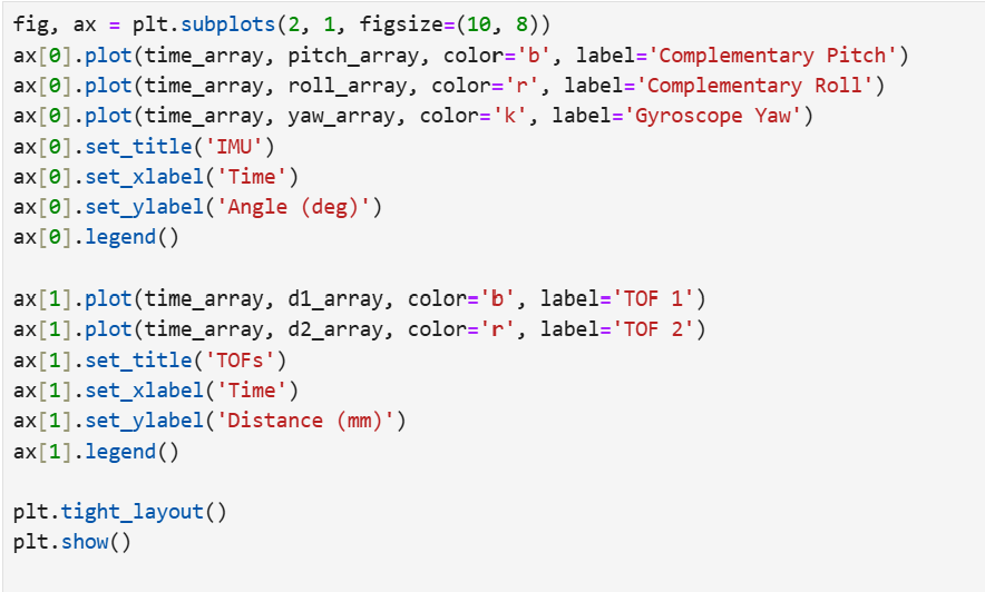
The notification handler and plotting code used for the 2 TOF case:
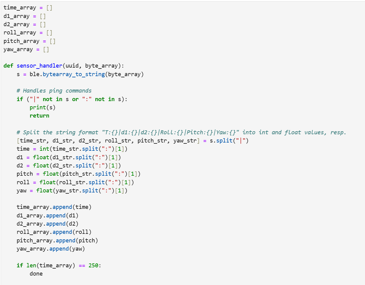
;