Lab 2: IMU

Prelab

The prelab involved reading up on the SparkFun IMU’s functionality and datasheet. My main takeaway from that was how the range of measurement on the Gyro and Accelerometer can be adjusted.

Setting Up the IMU

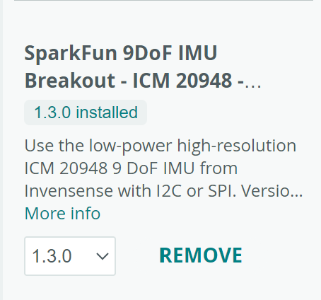
First, to set up the IMU, I installed the SparkFun 9DOF IMU Breakout_ICM 20948_Arduino Library in Arduino IDE.

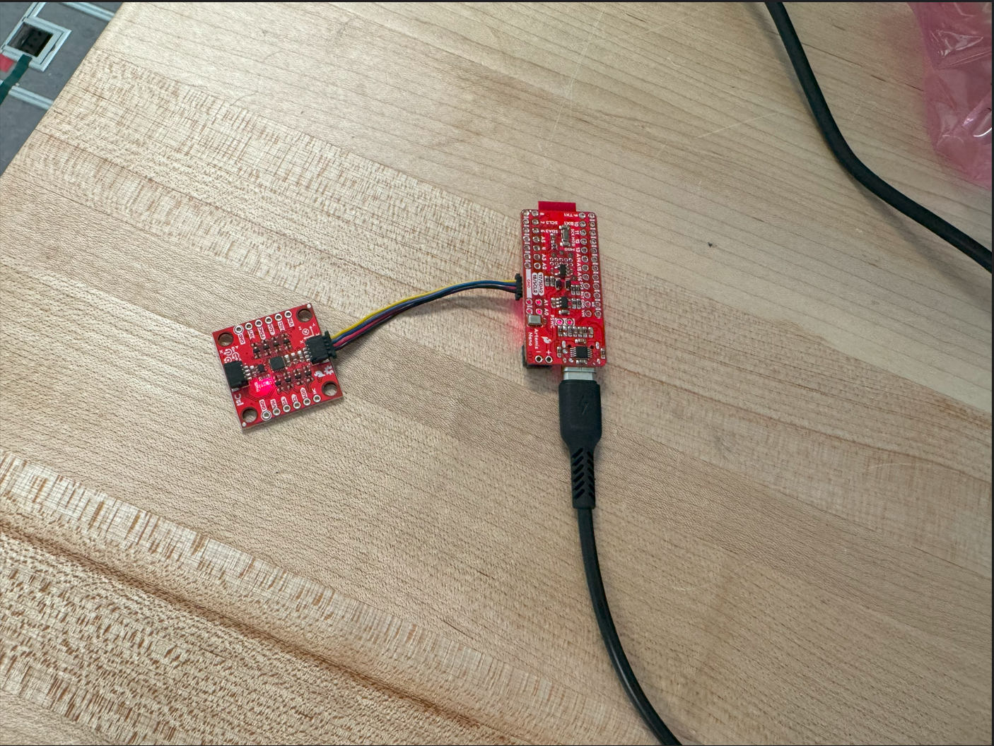
Then, I connected the IMU to my Artemis with the QWIIC cable as follows:

I burned the sketch ..\Arduino\libraries\SparkFun_ICM-20948\SparkFun_ICM-20948_ArduinoLibrary-master\examples\Arduino\Example1_Basics onto the Artemis. Upon keeping the serial monitor open for a minute, my Windows laptop immediately blue-screens. So I changed the baud rate from 115200 to 9600 to hopefully mitigate this issue. The serial plot shows the measurements from the accelerometer, which show constant values as I hold each axis up and down, which is expected because it measures the value of acceleration and gravity is the only acceleration acting on the board when I hold it in those directions. The serial monitor shows that the values for the gyroscope are non-zero when I begin rotating in each direction, which makes sense because it measures rotational rate. The video below shows me trying out the different outputs:

The value of the AD0_VAL pin should be 1 because the example code explicitly mentions that the default setting is 1 and it should only be changed to 0 if the ADR jumper becomes closed.

To complete the setup, I added a slow blink upon starting up the Artemis:

// Variables for the setup LED blinking
int ledState = LOW;
const int ledPin = LED_BUILTIN;  // the number of the LED pin
unsigned long previousMillis = 0; //last blink time
int ledInterval = 500; //If 0: don't blink; else: blink every [ledInterval] milliseconds
...
void ledStopBlink(){
  ledInterval = 0;
  digitalWrite(ledPin, LOW);
}
...
void ledCheckAndSet(){
  // To be called in loop(): handles checking LED state and turning it on/off to blink.

  // [ledInterval] == 0 if the LED should not blink.
  if (ledInterval){
    unsigned long currentMillis = millis();
    if (currentMillis - previousMillis >= ledInterval){
      previousMillis = currentMillis;

      //toggle state
      if (ledState == HIGH){
        ledState = LOW;
      } else {
        ledState = HIGH;
      }
    }
    digitalWrite(ledPin, ledState);
    
    // Three seconds after startup, stop blinking
    if (currentMillis > 3333){
      ledStopBlink();
    }
  }
}

The following video shows the blink in action:

Accelerometer

Calculate Pitch & Roll, Show at 0 and 90 Degrees

To convert the readings from the accelerometer into pitch and roll angles, I implemented the equations from class. We also want to take data quickly, so I decided to use the method of storing my IMU data points in a global array:

float theta = atan2((&myICM)->accX(), (&myICM)->accZ())  * (180.0 / M_PI);
float phi = atan2((&myICM)->accY(), (&myICM)->accZ()) * (180.0 / M_PI);
acc_pitch_array[i] = theta;
acc_roll_array[i] = phi;

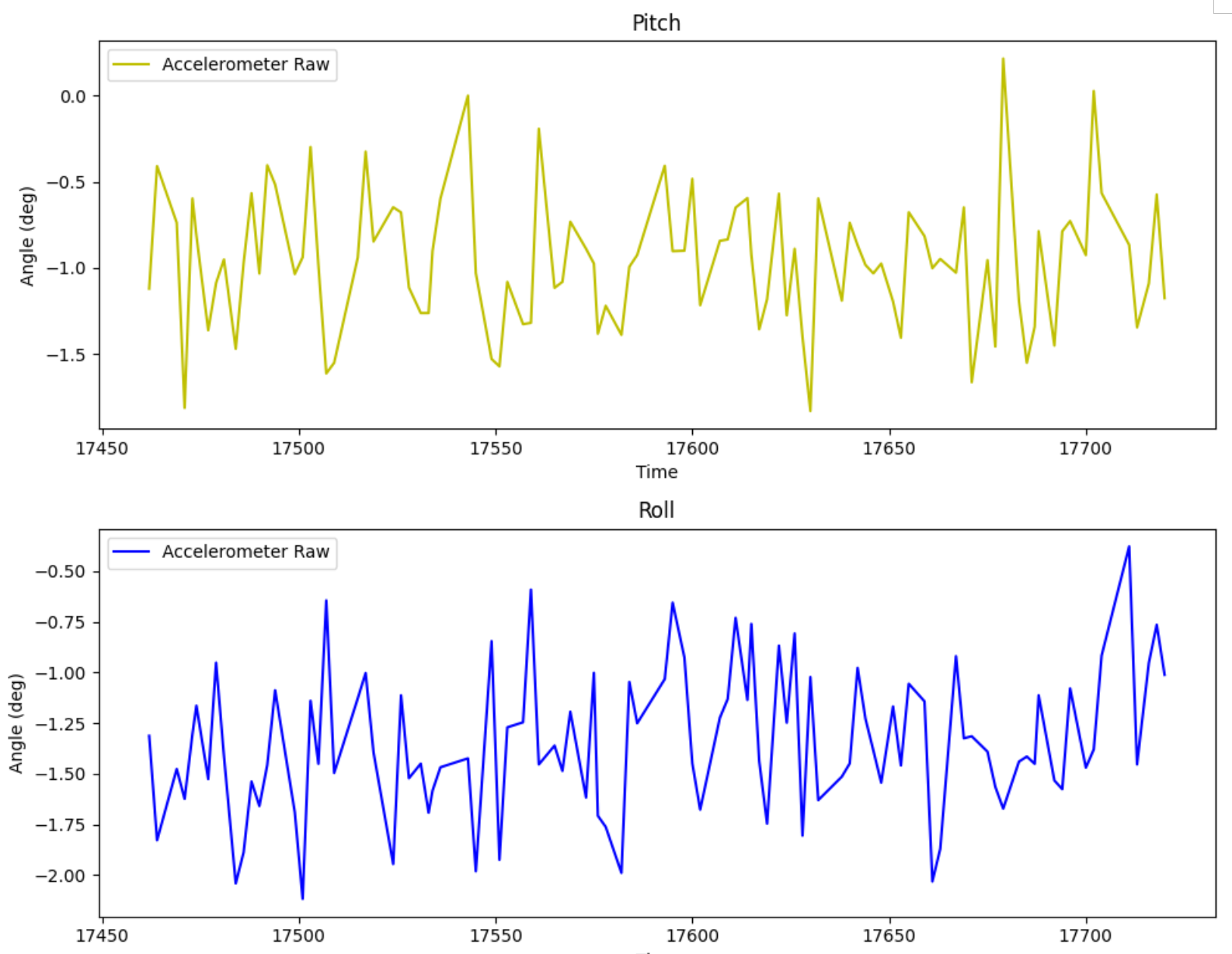
For pitch and roll, I laid the IMU flat for 0 degrees in both, and held it against the side of my box to read 90 degrees. The procedure is identical to what I did in the setup video. The graphs for each orientation are attached below.

Pitch = 0; Roll = 0:

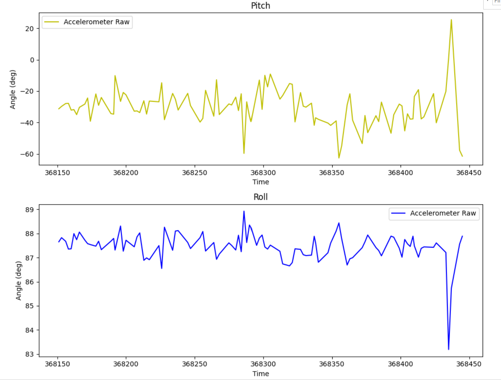
Pitch = 0; Roll = 90:

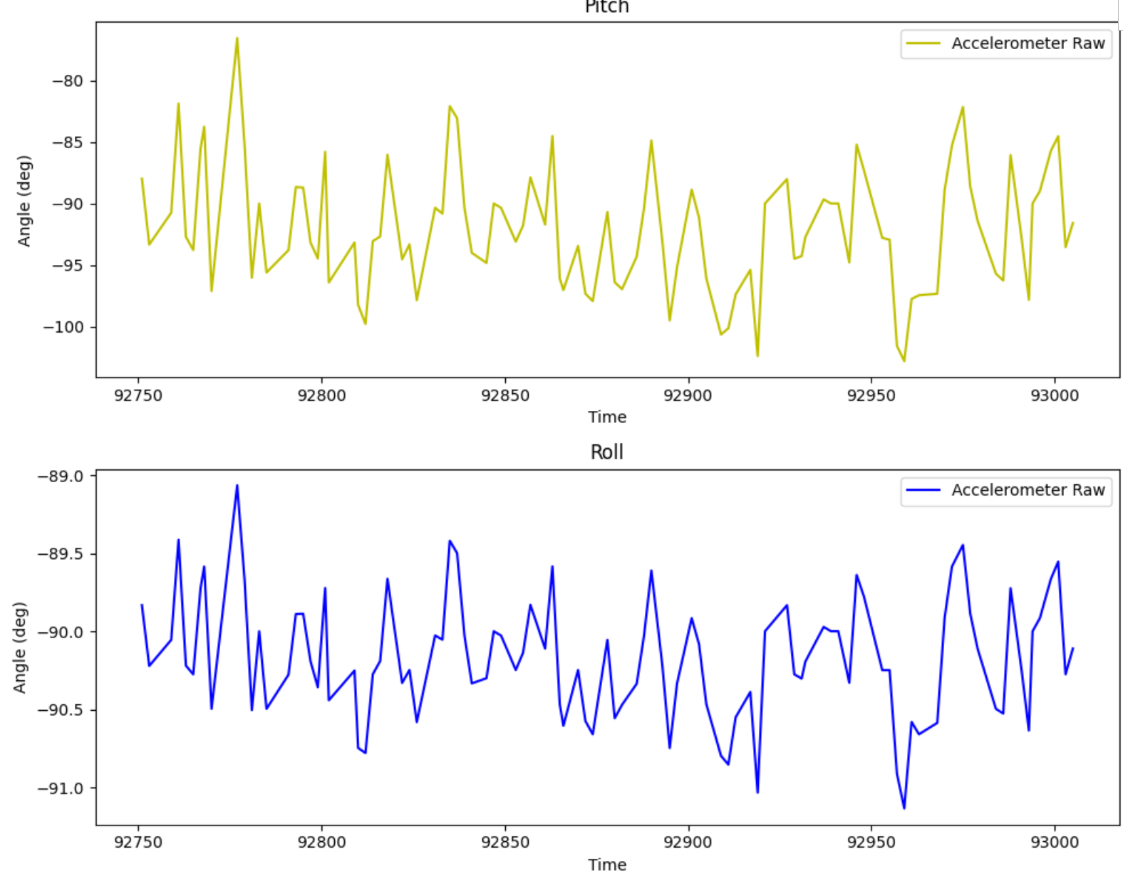
Pitch = 0; Roll = -90:

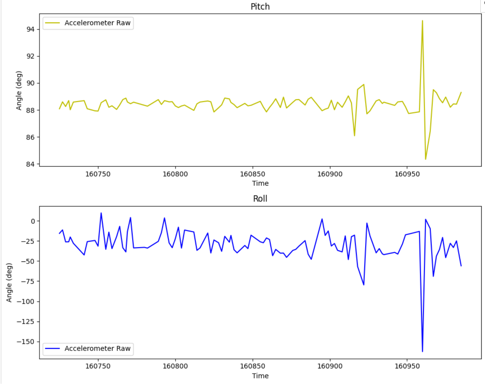
Pitch = 90; Roll = 0:

Pitch = -90; Roll = 0:

Note that when one angle is 90 degrees, gravity only acts in one component and the other reading becomes meaningless.

Two Point Calibration

Looking at the data above, I deemed that the accelerometer was accurate enough at 90 degrees on both extremes, both in pitch and roll. So while I did implement the two-point calibration (example function below), I did not use it in the following sections of the lab, and I probably will not use it going forward.

float calibratedRoll(float val){
  const float measuredMinus90 = -87.5;
  const float measuredPlus90 = 88; 

  return -90 + (val - measuredMinus90) * (180 / (measuredPlus90 - measuredMinus90));
}

float calibratedPitch(float val){
  const float measuredMinus90 = -85;
  const float measuredPlus90 = 87; 

  return -90 + (val - measuredMinus90) * (180 / (measuredPlus90 - measuredMinus90));
}

Recording Noise & FFT

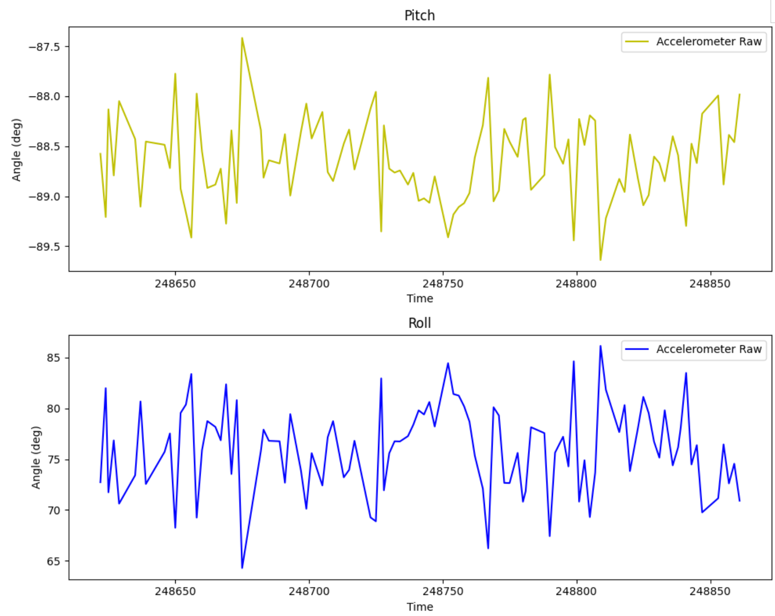
As we can see in the raw data, there is a lot of high frequency noise in the accelerometer, which oscillates within 1 degree of the mean value of the signal. I would have expected very little noise in these cases since the IMU is mostly stationary, and we saw in class that accelerometers usually are more noisy during movement. Observing this, it is clear that we need to implement a low pass filter in order to cut down on the noise which would only climb once we introduce movement.

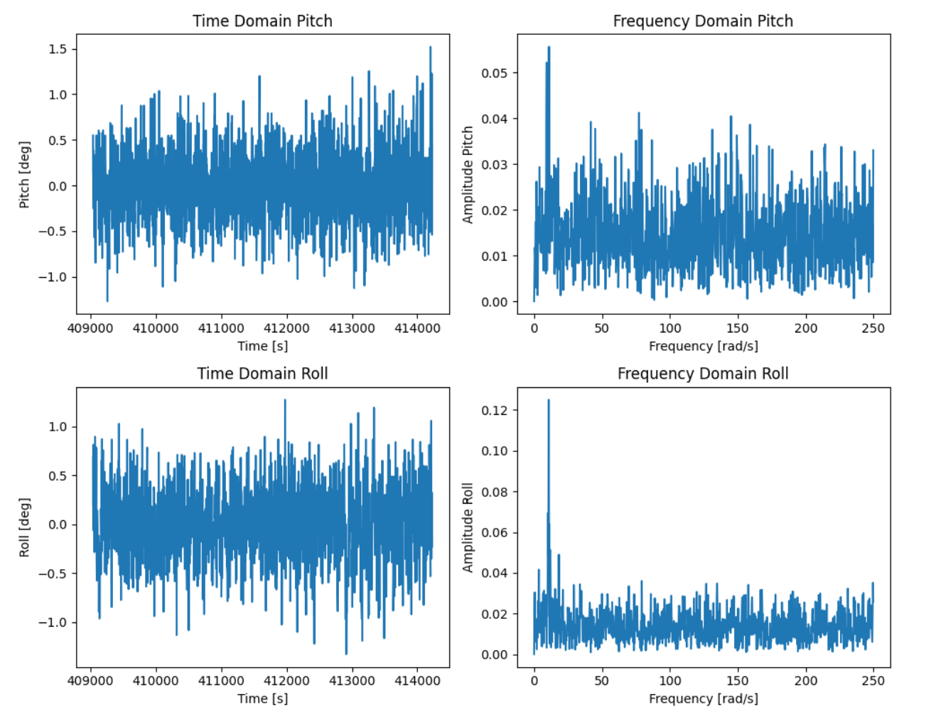
To analyze the noise on the accelerometer, I took data for two cases and computed the FFT for the data:

First, where the IMU is laying flat on the table:

Then, when the IMU is being vibrated by taps on the table:

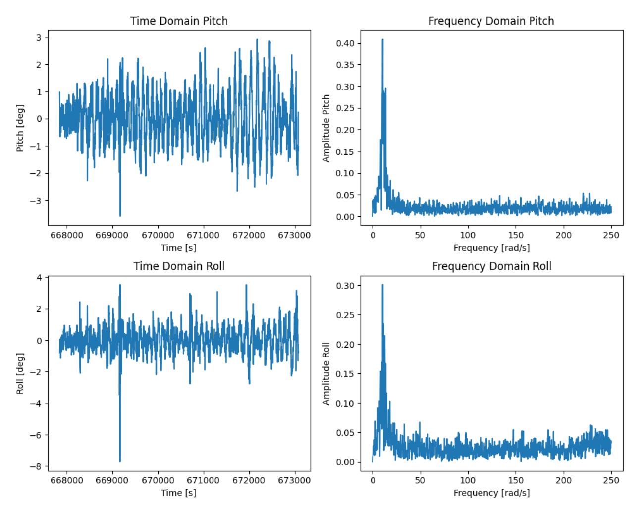
The cutoff frequency, as we can observe in the plot where the IMU is being tapped, is approximately 20 Hz. Using the equations from class, I can calculate an equivalent alpha:

$\alpha=\frac{T}{T+Rc}$ $T=\frac{1}{\text{sampling rate}}=\frac{1}{316.8}$ $f_c=\frac{1}{2 \pi RC} \implies RC = \frac{1}{2 \pi f_c}$ $\alpha = \frac{T}{T + \frac{1}{2 \pi f_c}} = \frac{316.8}{316.8 + \frac{1}{2 \pi * 20}} = 0.284$

Low Pass Filter

Plugging this into the Arduino implementation low pass filter. The code for pitch low pass is shown below, and it is identically copied for roll:

//Global Variables
const int array_size = 2000;
float acc_pitch_array_lowpass[array_size];
float lowpass_pitch[2];
const float alpha = 0.284;
...

float lowPassPitch(float val){
  if (!DO_LOWPASS) return val;

  bool isFirst = (lowpass_pitch == 0);

  lowpass_pitch[1] = alpha * val + (1 - alpha) * lowpass_pitch[0];
  lowpass_pitch[0] = lowpass_pitch[1]; 

  //To prevent large vertical spike from 0 -> first value
  if (isFirst) return val; 

  return lowpass_pitch[1];
}
...
for (int i = 0; i < array_size; i++){
  ...
  acc_pitch_array_lowpass[i] = lowPassPitch(theta);
  ...
}

I received the data and plotted in Jupyter, giving me:

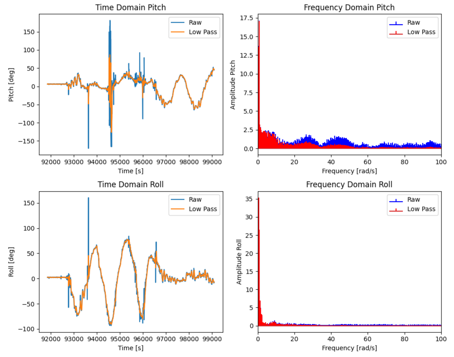
I can see that the higher frequency oscillations and noise were cut out, while the threshold was lenient enough to let the large spike in pitch (when I accidentally held it by the wire, dropping the IMU and causing a big spike) through to an extent.

Gyroscope

Computing RPY from Gyroscope

Since the gyroscope only calculates rates, we need to calculate pitch, roll, and yaw by using an integrator.

//Global variables
unsigned long gyr_last;
const int array_size = 2000;
float gyr_roll_array[array_size];
float gyr_pitch_array[array_size];
float gyr_yaw_array[array_size];

...
for (int i = 0; i < array_size; i++)
{
  ...
  // Initialization, on top of the CASE statement for BLE command
  float gyr_pitch = 0 , gyr_roll = 0, gyr_yaw = 0, dt = 0;
  gyr_last = micros();

  dt = ( micros() - gyr_last) / 1000000.;
  gyr_last = micros();
  gyr_pitch = gyr_pitch - myICM.gyrY()*dt; //negate gyro reading according to sign conv. defined on IMU
  gyr_roll = gyr_roll + myICM.gyrX()*dt;
  gyr_yaw = gyr_yaw + myICM.gyrZ()*dt;

  gyr_roll_array[i] = gyr_roll;
  gyr_pitch_array[i] = gyr_pitch; 
  gyr_yaw_array[i] = gyr_yaw;
  ...
}

Note that the pitch integrator is getting negated because I saw that the values for accelerometer and gyroscope pitch were opposite to each other. I checked the Y-axis definition on the board, and saw that the accelerometer was the one aligned correctly, so I negated the gyroscope pitch.

Gyroscope vs. Accelerometer

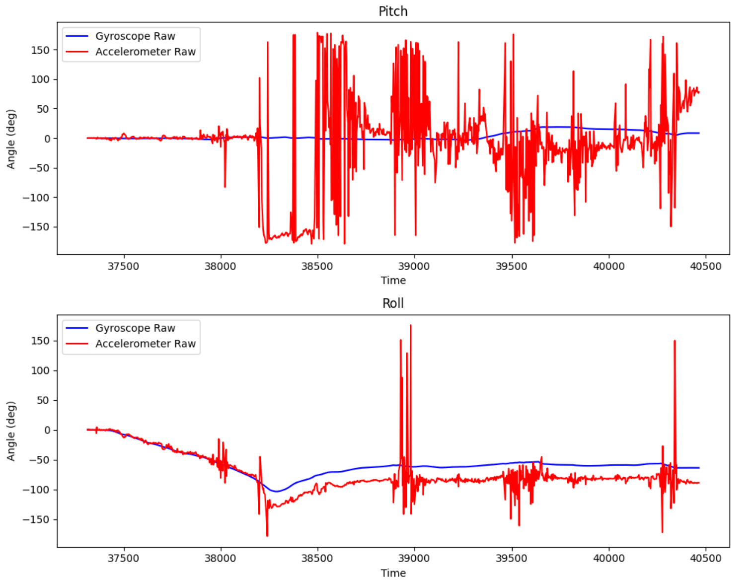
To show gyroscope at different positions, I only tested the cases where both pitch and roll are 0 degrees, and when either one is 90 degrees, just as a comparison to the accelerometer. I plotted both gyroscope and accelerometer readings on the same plot. An aside on why the graph starts at zero – I implemented the entire fetch-and-send flow in a BLE command, so I need to send the command, then move the IMU so that it can properly be initialized to 0 pitch and roll while flat on the ground.

Pitch = 0 ; Roll = 0:

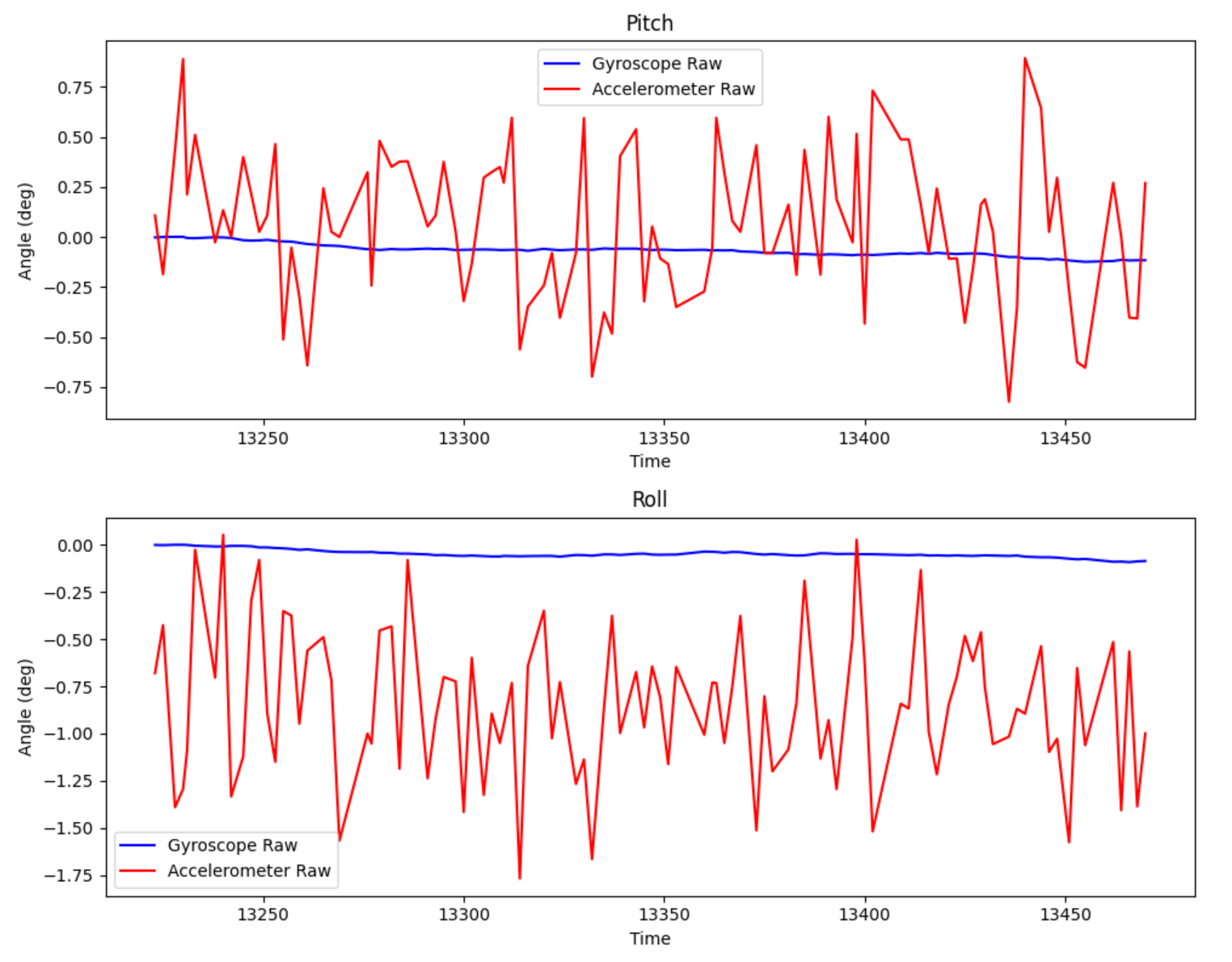
Pitch = 0; Roll = -90:

Pitch = 90; Roll = 0:

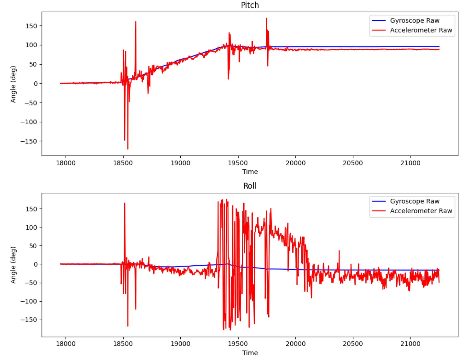
Generally speaking, the gyroscope has much less noise than the accelerometer reading. It is especially clear when quick movements are involved. During the 90 degree readings, me moving the IMU from flat to the end position caused massive accelerometer spikes, whereas the gyro was mainly stable throughout. However, the gyro reading deviates significantly from the mean value of the accelerometer, indicating drift.

Complementary Filter

To show the complementary filter, I used the equation from lecture, adding another integrator. Note that the gyroscope reading is negated for the same reason as above.

//Global Variables
const int array_size = 1000;
const float alpha_complementary = 0.1;
float complementary_pitch = 0, complementary_roll = 0;
float complementary_roll_array[array_size];
float complementary_pitch_array[array_size];

...

for (int i = 0; i < array_size; i++){
  dt = ( micros() - gyr_last) / 1000000.;
  gyr_last = micros();
  ...

  complementary_pitch = (complementary_pitch - myICM.gyrY()*dt)*(1-alpha_complementary) + theta * alpha_complementary; //also negate gyro
  complementary_roll = (complementary_roll + myICM.gyrX()*dt)*(1-alpha_complementary) + phi * alpha_complementary; 

  complementary_pitch_array[i] = complementary_pitch;
  complementary_roll_array[i] = complementary_roll;
}

To best test the range and effectiveness of the complementary filter, I will roll the IMU in both the roll and pitch directions, so that it hits 90 degrees on both sides. Then I will move it to an arbitrary angle in space and hold it there, to hopefully demonstrate some drift from the gyroscope.

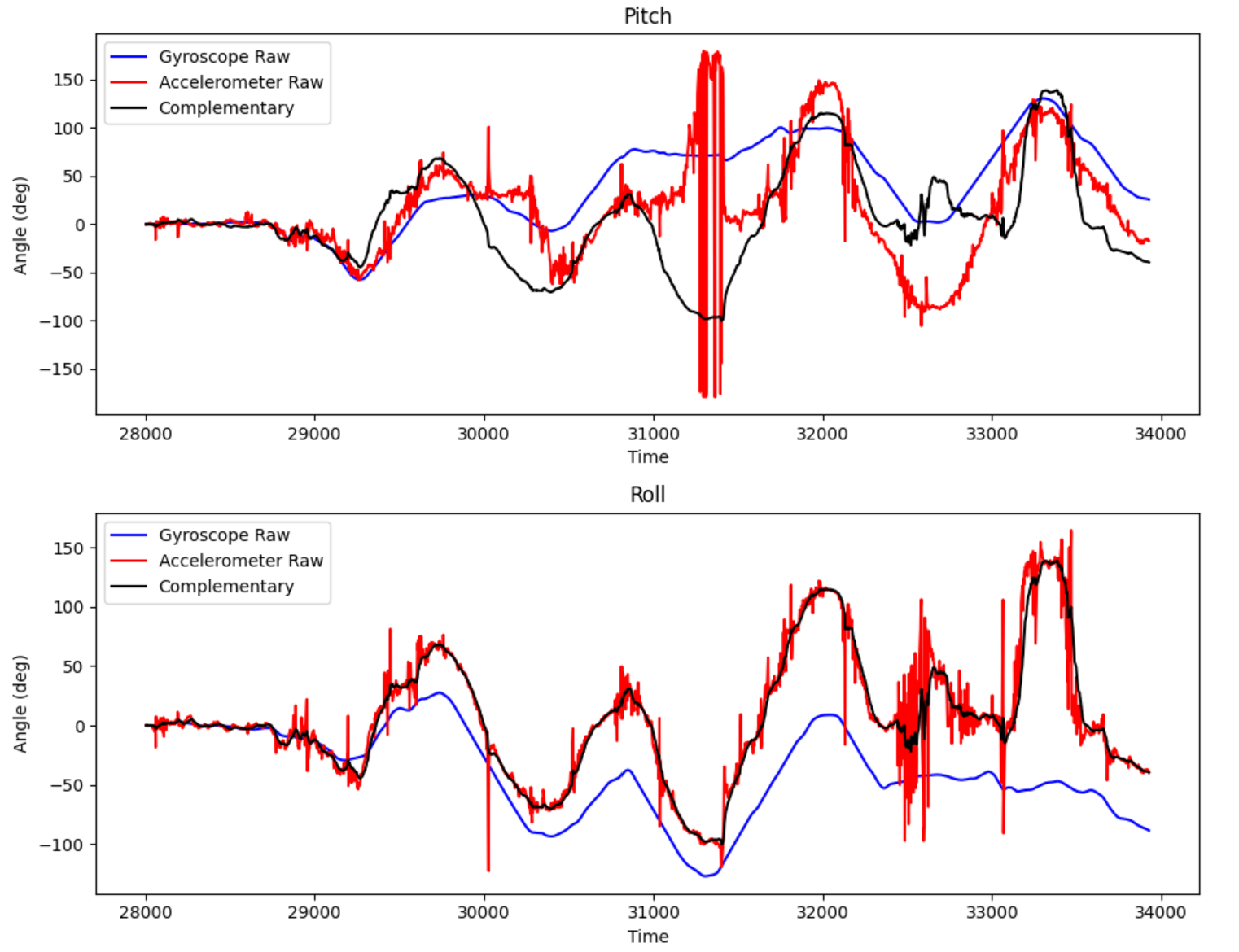
From this diagram we can see that the complementary filter can exceed +- 90 degrees whenever the accelerometer and gyroscope both do. Especially in the pitch direction, where I made sudden jerky movements, all of the sensor readings can be extreme.

The roll data, which is much more stable shows the gyroscope steadily has its mean value drifting far from the accelerometer value. However, the complementary reading is able to remove that drift. Also, the high frequency noise spikes in the accelerometer data is removed in the complementary signal, while the mean value is approximately preserved. This shows that the complementary filter is properly taking the strengths of both sensors in their fusion.

Sampling Data

Speed of Execution

Since we want code to execute as soon as possible on our robot, we shouldn’t block on when our code is ready. However, during my implementation in this lab, I put all of my fetch-and-send logic all in a bluetooth command. Since I didn’t use the main loop to execute the IMU readings, I couldn’t have intentionally blocked the execution of loop() with my code. I have also made sure there are no unnecessary slowdowns via delay() or Serial.print() statements.

One thing to note is that I tried to implement the code in a way where the main loop would continuously check and update values in global variables. A BLE command would trigger a write flag to write to arrays, then another BLE command would be used to fetch from the arrays in memory and send them to the processing computer. However, I couldn’t reconcile that with the fact that the main loop seems to block on execution of a BLE command, resulting in my attempt of that method to return only 0 in my arrays…

Storage of Data

As for how data is stored, I thought that separate arrays would be best for all types of data: gyro, accelerometer, complementary, and low pass. This primarily makes the code more modular and easier to understand. The only downside I could think of for this was potentially poor cache invalidation, where consecutive elements in an array would be cached together and therefore be faster to retrieve when sending it to the processing computer. (Although I am not sure the Nano even has a cache…)

The datatype used should always be the smallest size that can capture the precision needed. Certainly we can’t use ints because of the rounding issue. I chose floats, which tend to work well in my tests, because it is smaller than double.

Given that I stored 11 arrays of size 2000 in my global variables:

//Global Variables
const int array_size = 2000;
int timestamp_array[array_size];
float temperature_array[array_size];
float acc_roll_array[array_size];
float acc_pitch_array[array_size];

float gyr_roll_array[array_size];
float gyr_pitch_array[array_size];
float gyr_yaw_array[array_size];

float acc_roll_array_lowpass[array_size];
float acc_pitch_array_lowpass[array_size];

float complementary_roll_array[array_size];
float complementary_pitch_array[array_size];

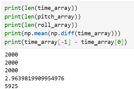
That should take up (11 arrays)(2000 elements)(4 bytes/float element) = 88000 and the Artemis upload returns: Global variables use 125296 bytes (31%) of dynamic memory, leaving 267920 bytes for local variables. Maximum is 393216 bytes., I could estimate the other global variables to take up about 40000 bytes. Removing that from the maximum, I have ~350000 bytes in total. If I did nothing else with the memory but add space in my array, then I could have 350000/(4 bytes * 11 arrays) ~= 7950 as my array size. On average, each element is ~3 ms apart, so it would correspond to ~23.8 seconds of data. The figure below shows the average time difference, and also shows that the last element is 5.9 seconds away from the first for a 2000 element array.

Stunts

Special thanks for Steven Sun for giving me the space and equipment to film these stunts. We collaborated on the stunts and used the best clips together. For an edited version, check out his video. Here are the raw clips that we recorded:

Casualty

Moment of silence for robot 1, who lost one of his legs during his brave stunt performances.

Discussion

In this lab I underwent the process of combining multiple sensors to leverage the strength of each individual sensor while eliminating their weaknesses. My biggest takeaway is how important it is to test each individual part before combining their readings, because once the system gets complex, any faulty component will have you searching blindly for a small mistake. I think this lab reinforced my understanding of timing in hardware-focused code, as in when I should declare and initialize my values. For example, if I had initialized all of my values for time using millis() in the global variables, I think the difference between the first and second data points would have been massive.

References

I referenced Mikayla Lahr’s website as a reference for what to include in my writeup. I also used her derivation for cutoff frequency after verifying it for myself.
Special thanks to Steven Sun for giving me a space to record my stunts, as well as letting me use his tripod and furniture for the stunts! He also helped me a great deal in debugging my FFT code, as well as debugging my integrator implementation.

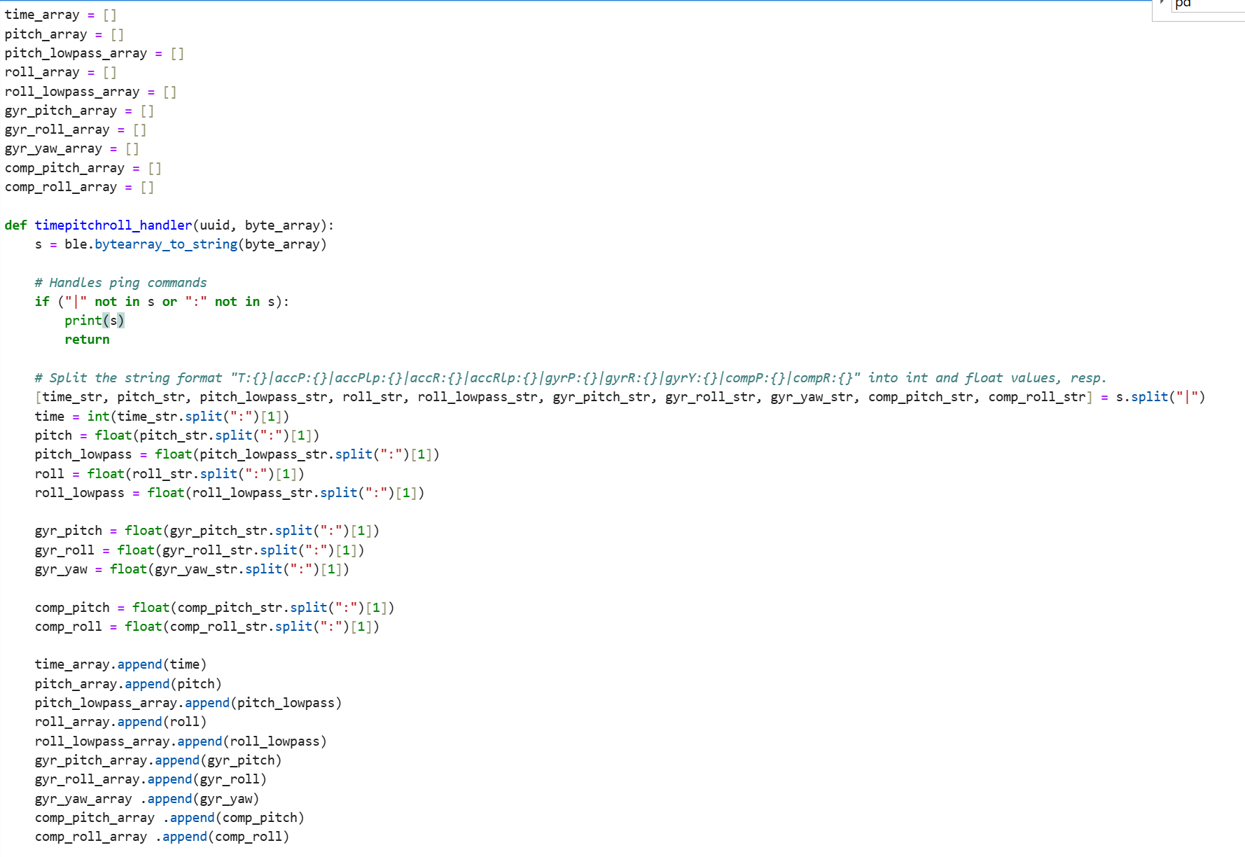
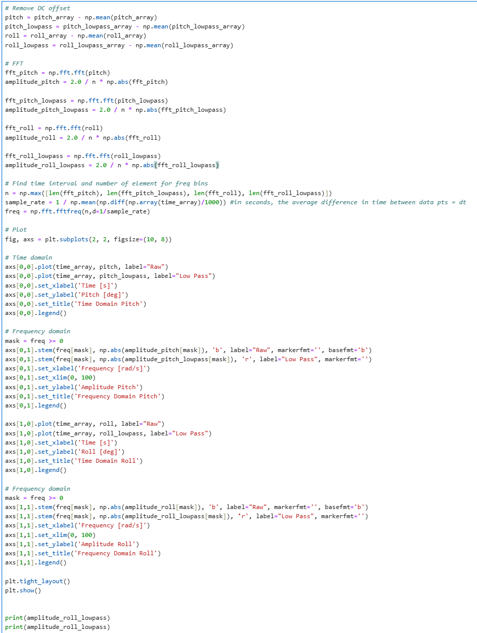
Appendix: Jupyter Code & FFT

Since I kept adding onto the same notification handler and FFT code, the resulting snippet became too long for the main writeup. I will add them here as a resource for future offerings of this class, if it is helpful.